Generative Modeling by Estimating Gradients of the Data Distribution

Introduction

Existing generative modeling techniques can largely be grouped into two categories based on how they represent probability distributions.

1. likelihood-based models, which directly learn the distribution’s probability density (or mass) function via (approximate) maximum likelihood. Typical likelihood-based models include autoregressive models , normalizing flow models , energy-based models (EBMs), and variational auto-encoders (VAEs) .
2. implicit generative models , where the probability distribution is implicitly represented by a model of its sampling process. The most prominent example is generative adversarial networks (GANs) , where new samples from the data distribution are synthesized by transforming a random Gaussian vector with a neural network.

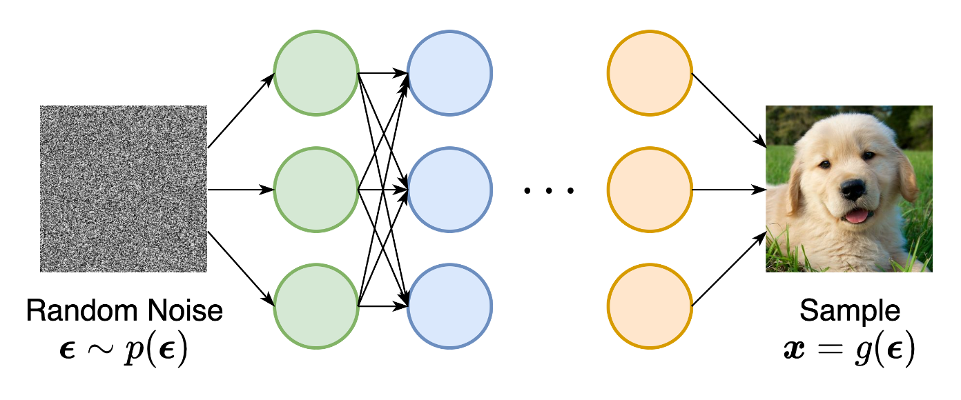
Likelihood-based models and implicit generative models, however, both have significant limitations. Likelihood-based models either require strong restrictions on the model architecture to ensure a tractable normalizing constant for likelihood computation, or must rely on surrogate objectives to approximate maximum likelihood training. Implicit generative models, on the other hand, often require adversarial training, which is notoriously unstable and can lead to mode collapse .

In this blog post, I will introduce another way to represent probability distributions that may circumvent several of these limitations. The key idea is to model the gradient of the log probability density function, a quantity often known as the (Stein) score function . Such score-based models are not required to have a tractable normalizing constant, and can be directly learned by score matching .

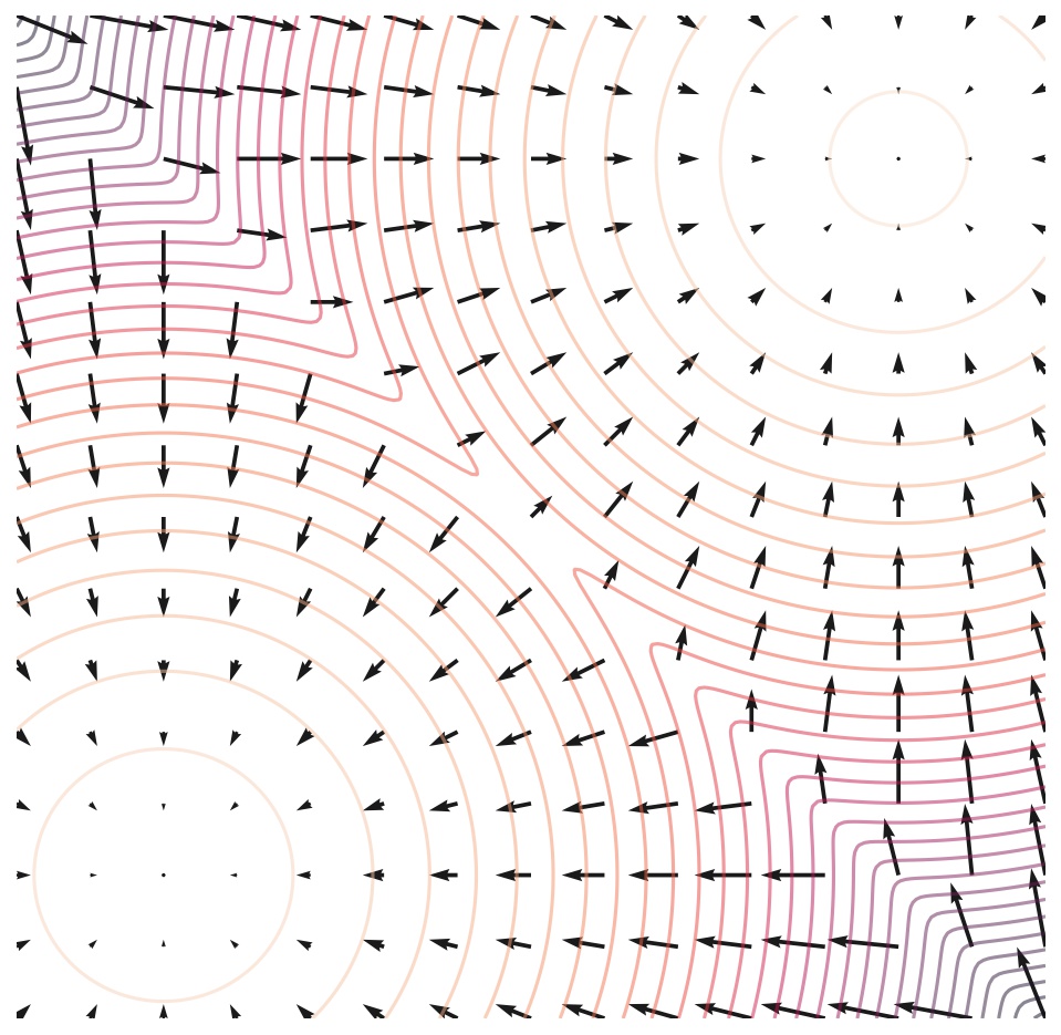
Score-based models have achieved state-of-the-art performance on many downstream tasks and applications. These tasks include, among others, image generation (Yes, better than GANs!), audio synthesis , shape generation, and music generation. Moreover, score-based models have connections to normalizing flow models, therefore allowing exact likelihood computation and representation learning. Additionally, modeling and estimating scores facilitates inverse problem solving, with applications such as image inpainting , image colorization , compressive sensing, and medical image reconstruction (e.g., CT, MRI) .

This post aims to show you the motivation and intuition of score-based generative modeling, as well as its basic concepts, properties and applications.

The score function, score-based models, and score matching

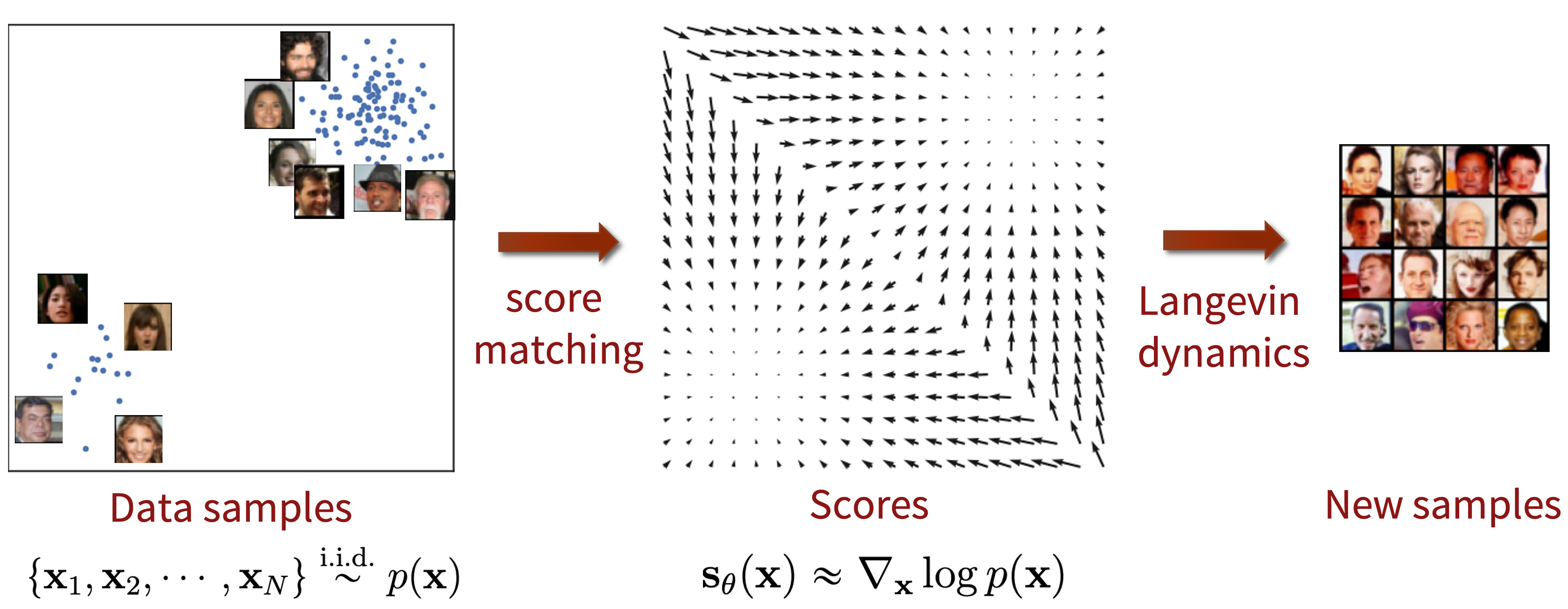
Suppose we are given a dataset \(\{\mathbf{x}_1, \mathbf{x}_2, \cdots, \mathbf{x}_N\}\), where each point is drawn independently from an underlying data distribution \(p(\mathbf{x})\). Given this dataset, the goal of generative modeling is to fit a model to the data distribution such that we can synthesize new data points at will by sampling from the distribution.

In order to build such a generative model, we first need a way to represent a probability distribution. One such way, as in likelihood-based models, is to directly model the probability density function (p.d.f.) or probability mass function (p.m.f.). Let \(f_\theta(\mathbf{x}) \in \mathbb{R}\) be a real-valued function parameterized by a learnable parameter \(\theta\). We can define a p.d.f. Hereafter we only consider probability density functions. Probability mass functions are similar. via \begin{align} p_\theta(\mathbf{x}) = \frac{e^{-f_\theta(\mathbf{x})}}{Z_\theta}, \label{ebm} \end{align} where \(Z_\theta > 0\) is a normalizing constant dependent on \(\theta\), such that \(\int p_\theta(\mathbf{x}) \textrm{d} \mathbf{x} = 1\). Here the function \(f_\theta(\mathbf{x})\) is often called an unnormalized probabilistic model, or energy-based model .

We can train \(p_\theta(\mathbf{x})\) by maximizing the log-likelihood of the data \begin{align} \max_\theta \sum_{i=1}^N \log p_\theta(\mathbf{x}_i). \label{mle} \end{align} However, equation \eqref{mle} requires \(p_\theta(\mathbf{x})\) to be a normalized probability density function. This is undesirable because in order to compute \(p_\theta(\mathbf{x})\), we must evaluate the normalizing constant \(Z_\theta\)—a typically intractable quantity for any general \(f_\theta(\mathbf{x})\). Thus to make maximum likelihood training feasible, likelihood-based models must either restrict their model architectures (e.g., causal convolutions in autoregressive models, invertible networks in normalizing flow models) to make \(Z_\theta\) tractable, or approximate the normalizing constant (e.g., variational inference in VAEs, or MCMC sampling used in contrastive divergence) which may be computationally expensive.

By modeling the score function instead of the density function, we can sidestep the difficulty of intractable normalizing constants. The score function of a distribution \(p(\mathbf{x})\) is defined as \begin{equation} \nabla_\mathbf{x} \log p(\mathbf{x}), \notag \end{equation} and a model for the score function is called a score-based model , which we denote as \(\mathbf{s}_\theta(\mathbf{x})\). The score-based model is learned such that \(\mathbf{s}_\theta(\mathbf{x}) \approx \nabla_\mathbf{x} \log p(\mathbf{x})\), and can be parameterized without worrying about the normalizing constant. For example, we can easily parameterize a score-based model with the energy-based model defined in equation \eqref{ebm} , via

Note that the score-based model \(\mathbf{s}_\theta(\mathbf{x})\) is independent of the normalizing constant \(Z_\theta\) ! This significantly expands the family of models that we can tractably use, since we don’t need any special architectures to make the normalizing constant tractable.

Similar to likelihood-based models, we can train score-based models by minimizing the Fisher divergence Fisher divergence is typically between two distributions p and q, defined as $$\begin{equation} \mathbb{E}_{p(\mathbf{x})}[\| \nabla_\mathbf{x} \log p(\mathbf{x}) - \nabla_\mathbf{x}\log q(\mathbf{x}) \|_2^2]. \end{equation}$$ Here we slightly abuse the term as the name of a closely related expression for score-based models. between the model and the data distributions, defined as \(\begin{equation} \mathbb{E}_{p(\mathbf{x})}[\| \nabla_\mathbf{x} \log p(\mathbf{x}) - \mathbf{s}_\theta(\mathbf{x}) \|_2^2]\label{fisher} \end{equation}\)

Intuitively, the Fisher divergence compares the squared \(\ell_2\) distance between the ground-truth data score and the score-based model. Directly computing this divergence, however, is infeasible because it requires access to the unknown data score \(\nabla_\mathbf{x} \log p(\mathbf{x})\). Fortunately, there exists a family of methods called score matching Commonly used score matching methods include denoising score matching and sliced score matching . Here is an introduction to score matching and sliced score matching. that minimize the Fisher divergence without knowledge of the ground-truth data score. Score matching objectives can directly be estimated on a dataset and optimized with stochastic gradient descent, analogous to the log-likelihood objective for training likelihood-based models (with known normalizing constants). We can train the score-based model by minimizing a score matching objective, without requiring adversarial optimization.

Additionally, using the score matching objective gives us a considerable amount of modeling flexibility. The Fisher divergence itself does not require \(\mathbf{s}_\theta(\mathbf{x})\) to be an actual score function of any normalized distribution—it simply compares the \(\ell_2\) distance between the ground-truth data score and the score-based model, with no additional assumptions on the form of \(\mathbf{s}_\theta(\mathbf{x})\). In fact, the only requirement on the score-based model is that it should be a vector-valued function with the same input and output dimensionality, which is easy to satisfy in practice.

As a brief summary, we can represent a distribution by modeling its score function, which can be estimated by training a score-based model of free-form architectures with score matching.

Langevin dynamics

Once we have trained a score-based model \(\mathbf{s}_\theta(\mathbf{x}) \approx \nabla_\mathbf{x} \log p(\mathbf{x})\), we can use an iterative procedure called Langevin dynamics to draw samples from it.

Langevin dynamics provides an MCMC procedure to sample from a distribution \(p(\mathbf{x})\) using only its score function \(\nabla_\mathbf{x} \log p(\mathbf{x})\). Specifically, it initializes the chain from an arbitrary prior distribution \(\mathbf{x}_0 \sim \pi(\mathbf{x})\), and then iterates the following

where \(\mathbf{z}_i \sim \mathcal{N}(0, I)\). When \(\epsilon \to 0\) and \(K \to \infty\), \(\mathbf{x}_K\) obtained from the procedure in \eqref{langevin} converges to a sample from \(p(\mathbf{x})\) under some regularity conditions. In practice, the error is negligible when \(\epsilon\) is sufficiently small and \(K\) is sufficiently large.

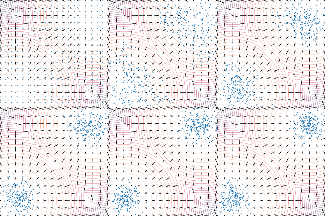
Note that Langevin dynamics accesses \(p(\mathbf{x})\) only through \(\nabla_\mathbf{x} \log p(\mathbf{x})\). Since \(\mathbf{s}_\theta(\mathbf{x}) \approx \nabla_\mathbf{x} \log p(\mathbf{x})\), we can produce samples from our score-based model \(\mathbf{s}_\theta(\mathbf{x})\) by plugging it into equation \eqref{langevin}.

Naive score-based generative modeling and its pitfalls

So far, we’ve discussed how to train a score-based model with score matching, and then produce samples via Langevin dynamics. However, this naive approach has had limited success in practice—we’ll talk about some pitfalls of score matching that received little attention in prior works.

The key challenge is the fact that the estimated score functions are inaccurate in low density regions, where few data points are available for computing the score matching objective. This is expected as score matching minimizes the Fisher divergence

Since the \(\ell_2\) differences between the true data score function and score-based model are weighted by \(p(\mathbf{x})\), they are largely ignored in low density regions where \(p(\mathbf{x})\) is small. This behavior can lead to subpar results, as illustrated by the figure below:

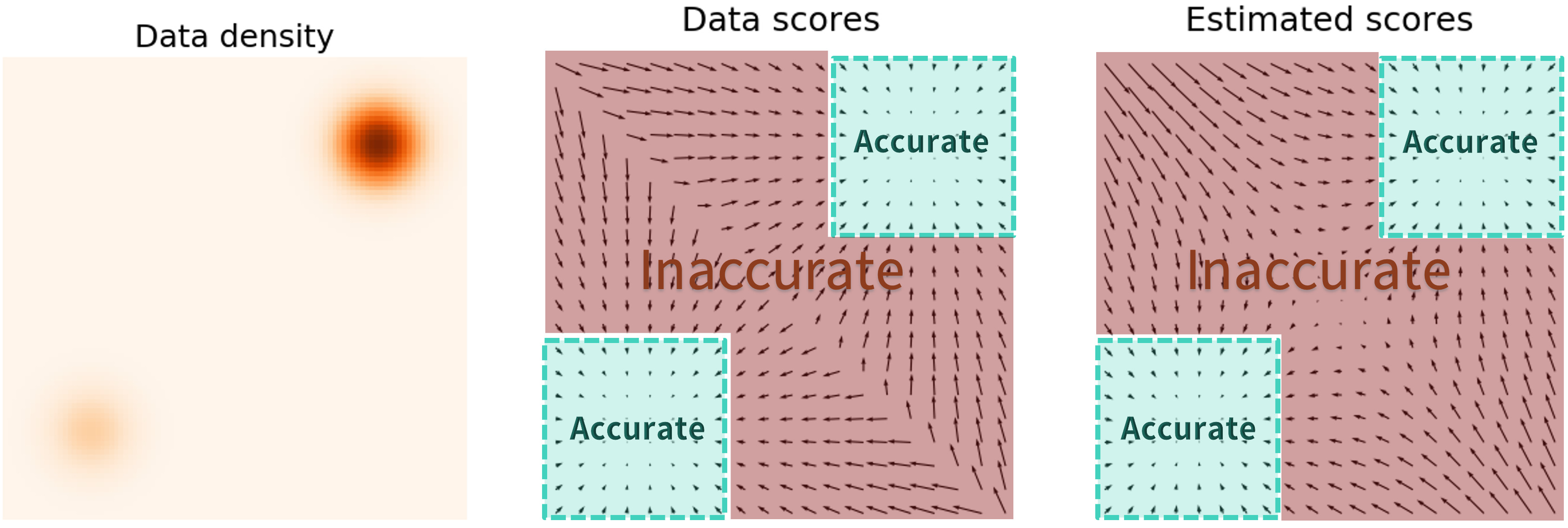
When sampling with Langevin dynamics, our initial sample is highly likely in low density regions when data reside in a high dimensional space. Therefore, having an inaccurate score-based model will derail Langevin dynamics from the very beginning of the procedure, preventing it from generating high quality samples that are representative of the data.

Score-based generative modeling with multiple noise perturbations

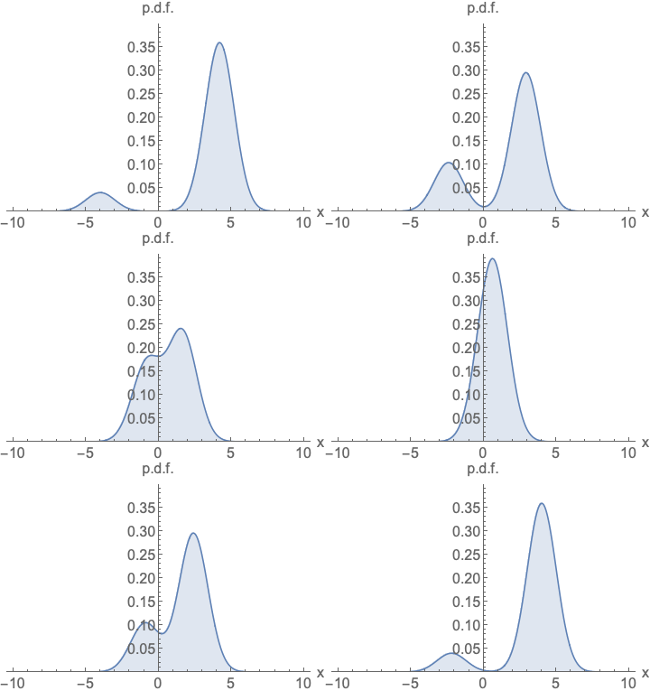
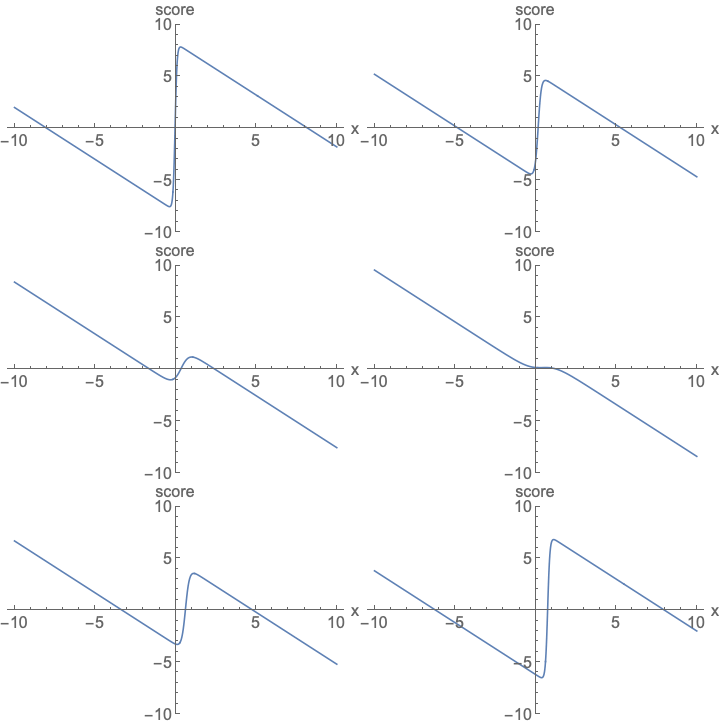
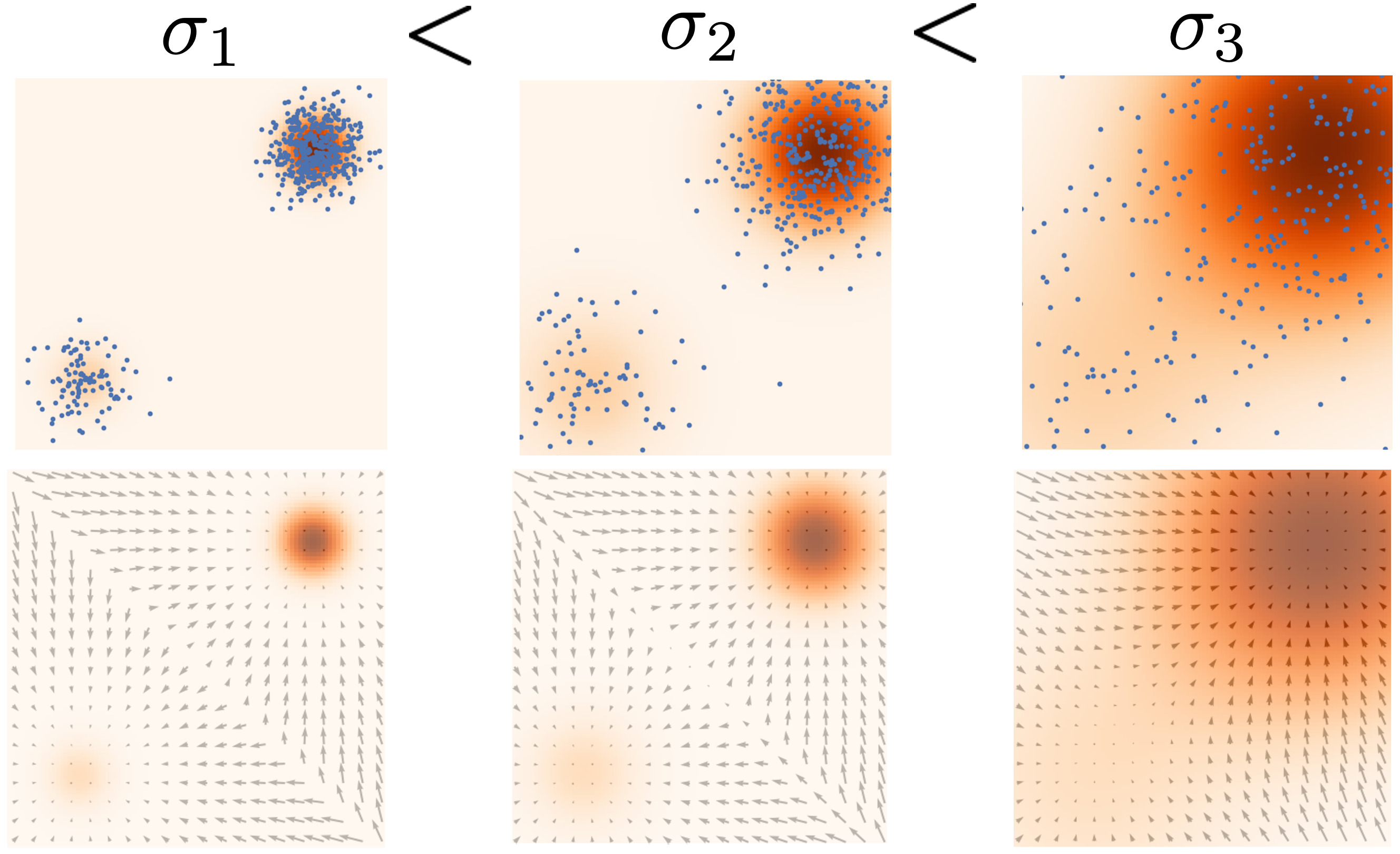
How can we bypass the difficulty of accurate score estimation in regions of low data density? Our solution is to perturb data points with noise and train score-based models on the noisy data points instead. When the noise magnitude is sufficiently large, it can populate low data density regions to improve the accuracy of estimated scores. For example, here is what happens when we perturb a mixture of two Gaussians perturbed by additional Gaussian noise.

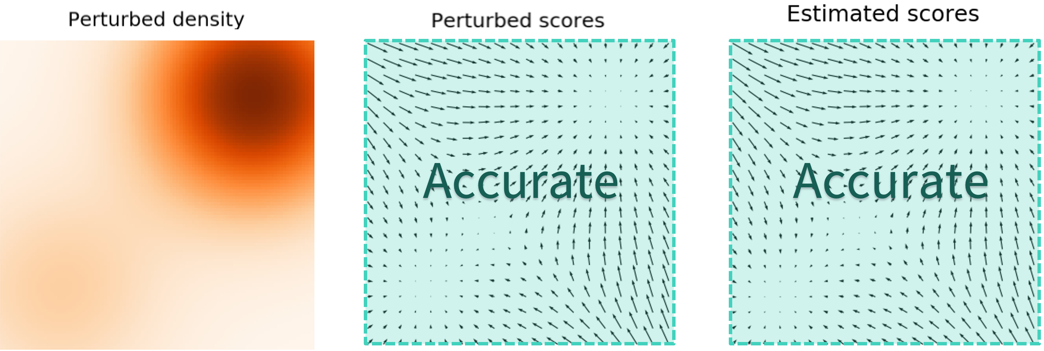
Yet another question remains: how do we choose an appropriate noise scale for the perturbation process? Larger noise can obviously cover more low density regions for better score estimation, but it over-corrupts the data and alters it significantly from the original distribution. Smaller noise, on the other hand, causes less corruption of the original data distribution, but does not cover the low density regions as well as we would like.

To achieve the best of both worlds, we use multiple scales of noise perturbations simultaneously . Suppose we always perturb the data with isotropic Gaussian noise, and let there be a total of \(L\) increasing standard deviations \(\sigma_1 < \sigma_2 < \cdots < \sigma_L\). We first perturb the data distribution \(p(\mathbf{x})\) with each of the Gaussian noise \(\mathcal{N}(0, \sigma_i^2 I), i=1,2,\cdots,L\) to obtain a noise-perturbed distribution

Note that we can easily draw samples from \(p_{\sigma_i}(\mathbf{x})\) by sampling \(\mathbf{x} \sim p(\mathbf{x})\) and computing \(\mathbf{x} + \sigma_i \mathbf{z}\), with \(\mathbf{z} \sim \mathcal{N}(0, I)\).

Next, we estimate the score function of each noise-perturbed distribution, \(\nabla_\mathbf{x} \log p_{\sigma_i}(\mathbf{x})\), by training a Noise Conditional Score-Based Model \(\mathbf{s}_\theta(\mathbf{x}, i)\) (also called a Noise Conditional Score Network, or NCSN, when parameterized with a neural network) with score matching, such that \(\mathbf{s}_\theta(\mathbf{x}, i) \approx \nabla_\mathbf{x} \log p_{\sigma_i}(\mathbf{x})\) for all \(i= 1, 2, \cdots, L\).

The training objective for \(\mathbf{s}_\theta(\mathbf{x}, i)\) is a weighted sum of Fisher divergences for all noise scales. In particular, we use the objective below:

where \(\lambda(i) \in \mathbb{R}_{>0}\) is a positive weighting function, often chosen to be \(\lambda(i) = \sigma_i^2\). The objective \eqref{ncsn_obj} can be optimized with score matching, exactly as in optimizing the naive (unconditional) score-based model \(\mathbf{s}_\theta(\mathbf{x})\).

After training our noise-conditional score-based model \(\mathbf{s}_\theta(\mathbf{x}, i)\), we can produce samples from it by running Langevin dynamics for \(i = L, L-1, \cdots, 1\) in sequence. This method is called annealed Langevin dynamics (defined by Algorithm 1 in , and improved by ), since the noise scale \(\sigma_i\) decreases (anneals) gradually over time.

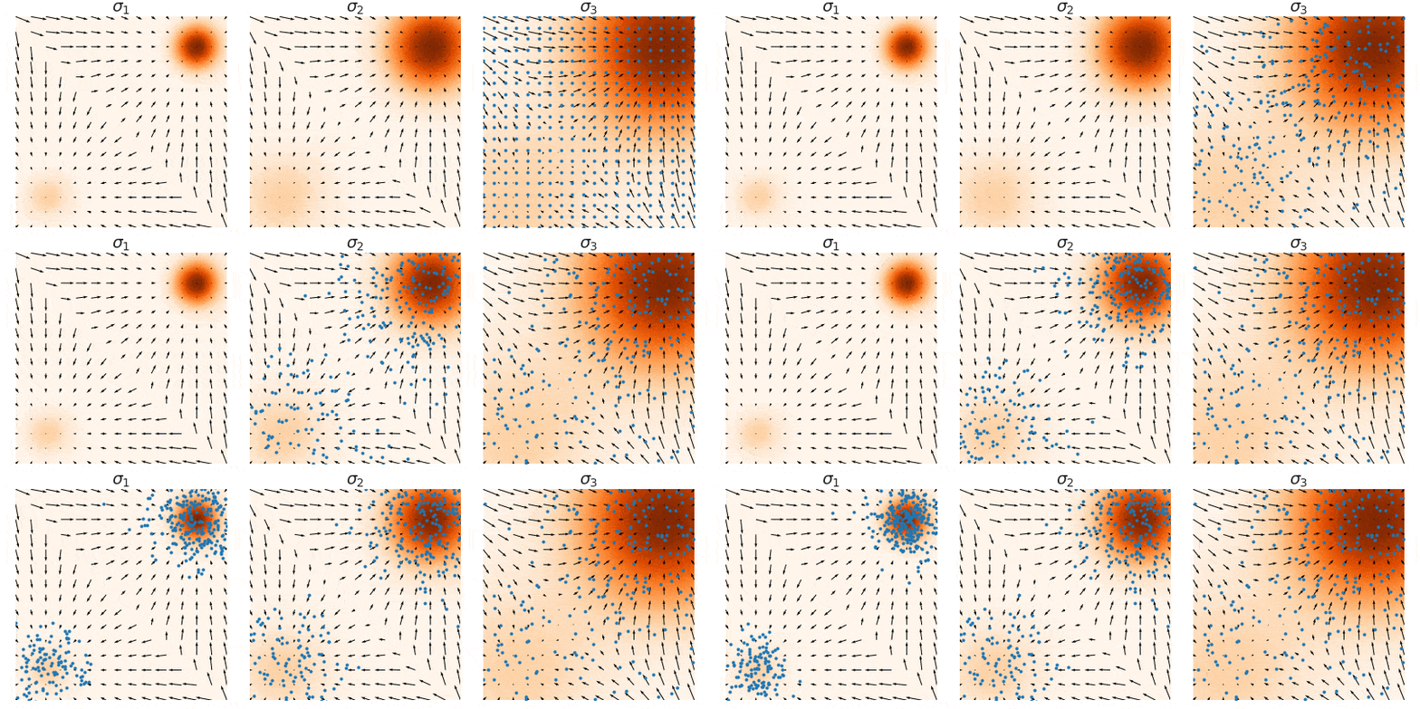
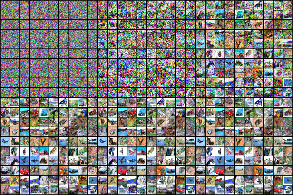
Here are some practical recommendations for tuning score-based generative models with multiple noise scales:

• Choose \(\sigma_1 < \sigma_2 < \cdots < \sigma_L\) as a geometric progression, with \(\sigma_1\) being sufficiently small and \(\sigma_L\) comparable to the maximum pairwise distance between all training data points . \(L\) is typically on the order of hundreds or thousands.

• Parameterize the score-based model \(\mathbf{s}_\theta(\mathbf{x}, i)\) with U-Net skip connections .

• Apply exponential moving average on the weights of the score-based model when used at test time .

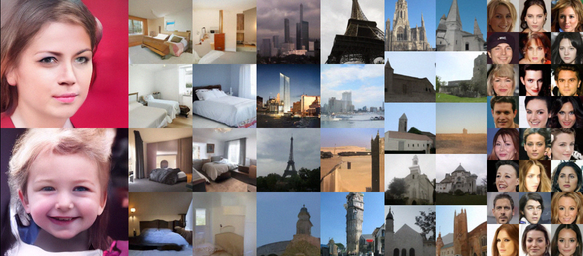
With such best practices, we are able to generate high quality image samples with comparable quality to GANs on various datasets, such as below:

Score-based generative modeling with stochastic differential equations (SDEs)

As we already discussed, adding multiple noise scales is critical to the success of score-based generative models. By generalizing the number of noise scales to infinity , we obtain not only higher quality samples, but also, among others, exact log-likelihood computation, and controllable generation for inverse problem solving.

In addition to this introduction, we have tutorials written in Google Colab to provide a step-by-step guide for training a toy model on MNIST. We also have more advanced code repositories that provide full-fledged implementations for large scale applications.

Link	Description
	Tutorial of score-based generative modeling with SDEs in JAX + FLAX
	Load our pretrained checkpoints and play with sampling, likelihood computation, and controllable synthesis (JAX + FLAX)
	Tutorial of score-based generative modeling with SDEs in PyTorch
	Load our pretrained checkpoints and play with sampling, likelihood computation, and controllable synthesis (PyTorch)
Code in JAX	Score SDE codebase in JAX + FLAX
Code in PyTorch	Score SDE codebase in PyTorch

Perturbing data with an SDE

When the number of noise scales approaches infinity, we essentially perturb the data distribution with continuously growing levels of noise. In this case, the noise perturbation procedure is a continuous-time stochastic process, as demonstrated below

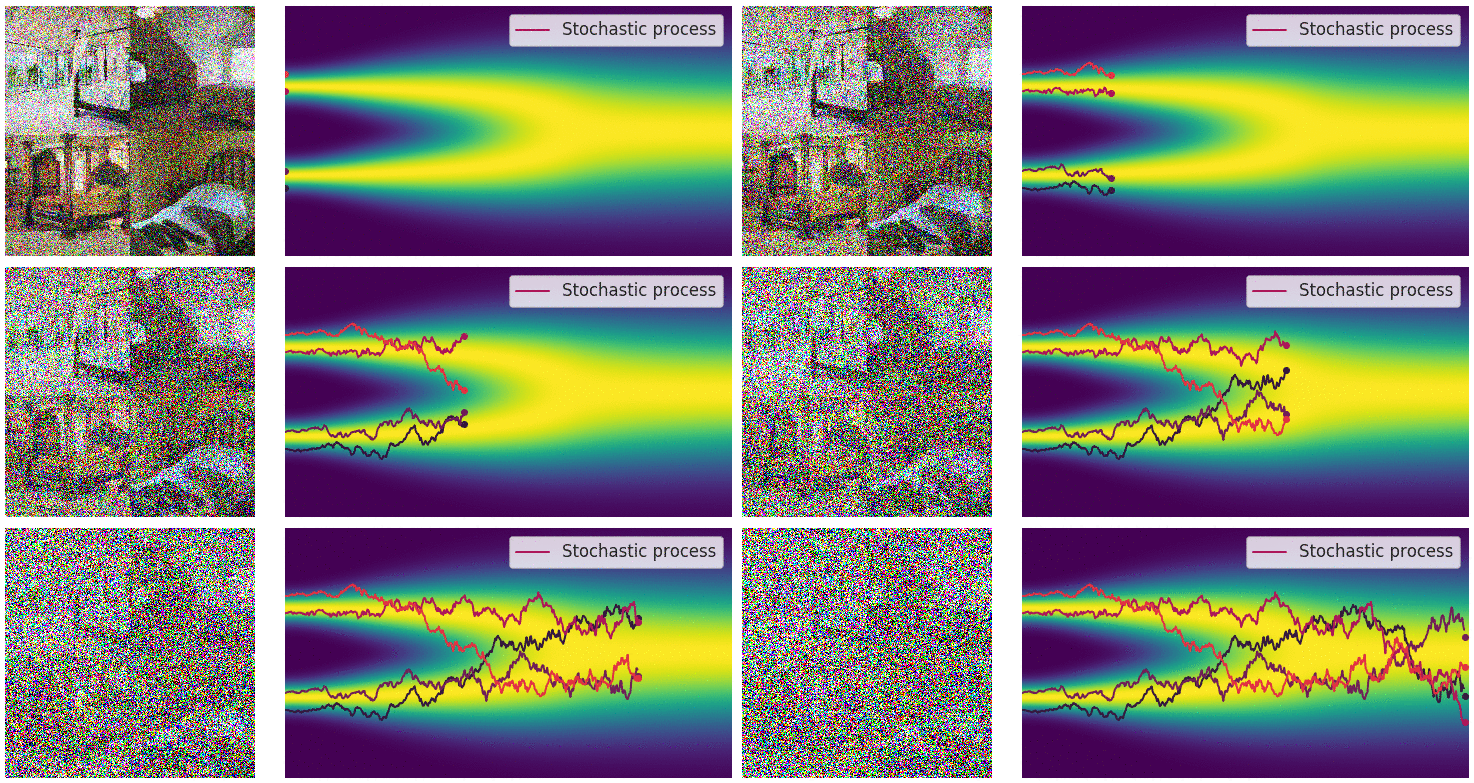
How can we represent a stochastic process in a concise way? Many stochastic processes (diffusion processes in particular) are solutions of stochastic differential equations (SDEs). In general, an SDE possesses the following form:

where \(\mathbf{f}(\cdot, t): \mathbb{R}^d \to \mathbb{R}^d\) is a vector-valued function called the drift coefficient, \(g(t)\in \mathbb{R}\) is a real-valued function called the diffusion coefficient, \(\mathbf{w}\) denotes a standard Brownian motion, and \(\mathrm{d} \mathbf{w}\) can be viewed as infinitesimal white noise. The solution of a stochastic differential equation is a continuous collection of random variables \(\{ \mathbf{x}(t) \}_{t\in [0, T]}\). These random variables trace stochastic trajectories as the time index \(t\) grows from the start time \(0\) to the end time \(T\). Let \(p_t(\mathbf{x})\) denote the (marginal) probability density function of \(\mathbf{x}(t)\). Here \(t \in [0, T]\) is analogous to \(i = 1, 2, \cdots, L\) when we had a finite number of noise scales, and \(p_t(\mathbf{x})\) is analogous to \(p_{\sigma_i}(\mathbf{x})\). Clearly, \(p_0(\mathbf{x}) = p(\mathbf{x})\) is the data distribution since no perturbation is applied to data at \(t=0\). After perturbing \(p(\mathbf{x})\) with the stochastic process for a sufficiently long time \(T\), \(p_T(\mathbf{x})\) becomes close to a tractable noise distribution \(\pi(\mathbf{x})\), called a prior distribution. We note that \(p_T(\mathbf{x})\) is analogous to \(p_{\sigma_L}(\mathbf{x})\) in the case of finite noise scales, which corresponds to applying the largest noise perturbation \(\sigma_L\) to the data.

The SDE in \eqref{sde} is hand designed, similarly to how we hand-designed \(\sigma_1 < \sigma_2 < \cdots < \sigma_L\) in the case of finite noise scales. There are numerous ways to add noise perturbations, and the choice of SDEs is not unique. For example, the following SDE

perturbs data with a Gaussian noise of mean zero and exponentially growing variance, which is analogous to perturbing data with \(\mathcal{N}(0, \sigma_1^2 I), \mathcal{N}(0, \sigma_2^2 I), \cdots, \mathcal{N}(0, \sigma_L^2 I)\) when \(\sigma_1 < \sigma_2 < \cdots < \sigma_L\) is a geometric progression. Therefore, the SDE should be viewed as part of the model, much like \(\{\sigma_1, \sigma_2, \cdots, \sigma_L\}\). In , we provide three SDEs that generally work well for images: the Variance Exploding SDE (VE SDE), the Variance Preserving SDE (VP SDE), and the sub-VP SDE.

Reversing the SDE for sample generation

Recall that with a finite number of noise scales, we can generate samples by reversing the perturbation process with annealed Langevin dynamics, i.e., sequentially sampling from each noise-perturbed distribution using Langevin dynamics. For infinite noise scales, we can analogously reverse the perturbation process for sample generation by using the reverse SDE.

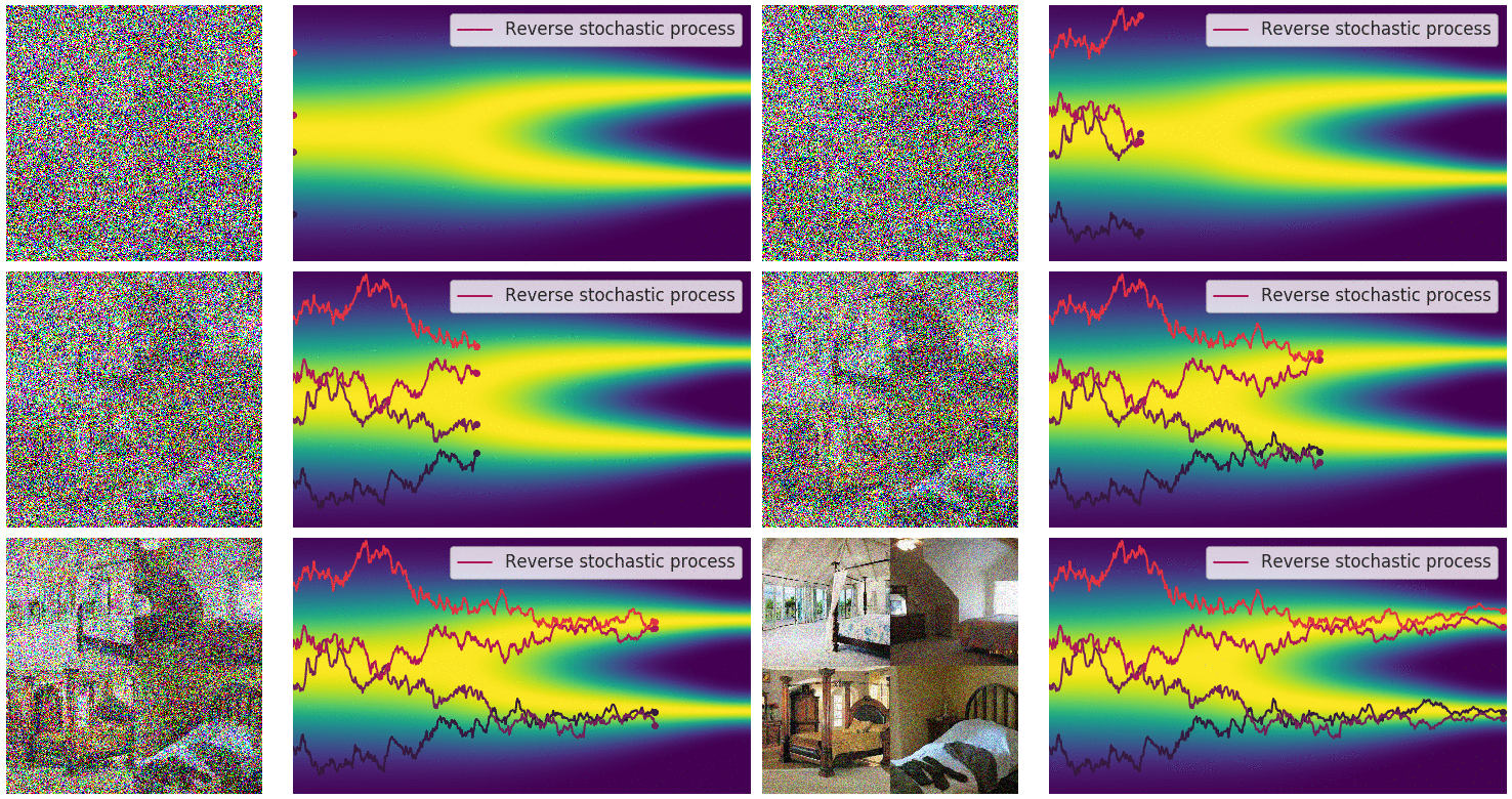
Importantly, any SDE has a corresponding reverse SDE , whose closed form is given by

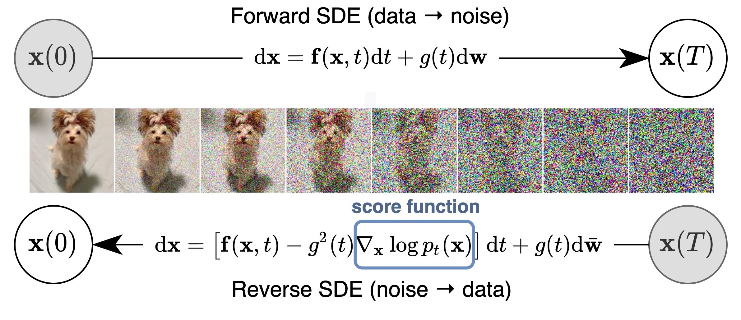
Here \(\mathrm{d} t\) represents a negative infinitesimal time step, since the SDE \eqref{rsde} needs to be solved backwards in time (from \(t=T\) to \(t = 0\)). In order to compute the reverse SDE, we need to estimate \(\nabla_\mathbf{x} \log p_t(\mathbf{x})\), which is exactly the score function of \(p_t(\mathbf{x})\).

Estimating the reverse SDE with score-based models and score matching

Solving the reverse SDE requires us to know the terminal distribution \(p_T(\mathbf{x})\), and the score function \(\nabla_\mathbf{x} \log p_t(\mathbf{x})\). By design, the former is close to the prior distribution \(\pi(\mathbf{x})\) which is fully tractable. In order to estimate \(\nabla_\mathbf{x} \log p_t(\mathbf{x})\), we train a Time-Dependent Score-Based Model \(\mathbf{s}_\theta(\mathbf{x}, t)\), such that \(\mathbf{s}_\theta(\mathbf{x}, t) \approx \nabla_\mathbf{x} \log p_t(\mathbf{x})\). This is analogous to the noise-conditional score-based model \(\mathbf{s}_\theta(\mathbf{x}, i)\) used for finite noise scales, trained such that \(\mathbf{s}_\theta(\mathbf{x}, i) \approx \nabla_\mathbf{x} \log p_{\sigma_i}(\mathbf{x})\).

Our training objective for \(\mathbf{s}_\theta(\mathbf{x}, t)\) is a continuous weighted combination of Fisher divergences, given by

where \(\mathcal{U}(0, T)\) denotes a uniform distribution over the time interval \([0, T]\), and \(\lambda: \mathbb{R} \to \mathbb{R}_{>0}\) is a positive weighting function. Typically we use \(\lambda(t) \propto 1/ \mathbb{E}[\| \nabla_{\mathbf{x}(t)} \log p(\mathbf{x}(t) \mid \mathbf{x}(0))\|_2^2]\) to balance the magnitude of different score matching losses across time.

As before, our weighted combination of Fisher divergences can be efficiently optimized with score matching methods, such as denoising score matching and sliced score matching . Once our score-based model \(\mathbf{s}_\theta(\mathbf{x}, t)\) is trained to optimality, we can plug it into the expression of the reverse SDE in \eqref{rsde} to obtain an estimated reverse SDE.

We can start with \(\mathbf{x}(T) \sim \pi\), and solve the above reverse SDE to obtain a sample \(\mathbf{x}(0)\). Let us denote the distribution of \(\mathbf{x}(0)\) obtained in such way as \(p_\theta\). When the score-based model \(\mathbf{s}_\theta(\mathbf{x}, t)\) is well-trained, we have \(p_\theta \approx p_0\), in which case \(\mathbf{x}(0)\) is an approximate sample from the data distribution \(p_0\).

When \(\lambda(t) = g^2(t)\), we have an important connection between our weighted combination of Fisher divergences and the KL divergence from \(p_0\) to \(p_\theta\) under some regularity conditions :

Due to this special connection to the KL divergence and the equivalence between minimizing KL divergences and maximizing likelihood for model training, we call \(\lambda(t) = g(t)^2\) the likelihood weighting function. Using this likelihood weighting function, we can train score-based generative models to achieve very high likelihoods, comparable or even superior to state-of-the-art autoregressive models.

How to solve the reverse SDE

By solving the estimated reverse SDE with numerical SDE solvers, we can simulate the reverse stochastic process for sample generation. Perhaps the simplest numerical SDE solver is the Euler-Maruyama method. When applied to our estimated reverse SDE, it discretizes the SDE using finite time steps and small Gaussian noise. Specifically, it chooses a small negative time step \(\Delta t \approx 0\), initializes \(t \gets T\), and iterates the following procedure until \(t \approx 0\):

Here \(\mathbf{z}_t \sim \mathcal{N}(0, I)\). The Euler-Maruyama method is qualitatively similar to Langevin dynamics—both update \(\mathbf{x}\) by following score functions perturbed with Gaussian noise.

Aside from the Euler-Maruyama method, other numerical SDE solvers can be directly employed to solve the reverse SDE for sample generation, including, for example, Milstein method, and stochastic Runge-Kutta methods. In , we provided a reverse diffusion solver similar to Euler-Maruyama, but more tailored for solving reverse-time SDEs. More recently, authors in introduced adaptive step-size SDE solvers that can generate samples faster with better quality.

In addition, there are two special properties of our reverse SDE that allow for even more flexible sampling methods:

• We have an estimate of \(\nabla_\mathbf{x} \log p_t(\mathbf{x})\) via our time-dependent score-based model \(\mathbf{s}_\theta(\mathbf{x}, t)\).
• We only care about sampling from each marginal distribution \(p_t(\mathbf{x})\). Samples obtained at different time steps can have arbitrary correlations and do not have to form a particular trajectory sampled from the reverse SDE.

As a consequence of these two properties, we can apply MCMC approaches to fine-tune the trajectories obtained from numerical SDE solvers. Specifically, we propose Predictor-Corrector samplers. The predictor can be any numerical SDE solver that predicts \(\mathbf{x}(t + \Delta t) \sim p_{t+\Delta t}(\mathbf{x})\) from an existing sample \(\mathbf{x}(t) \sim p_t(\mathbf{x})\). The corrector can be any MCMC procedure that solely relies on the score function, such as Langevin dynamics and Hamiltonian Monte Carlo.

At each step of the Predictor-Corrector sampler, we first use the predictor to choose a proper step size \(\Delta t < 0\), and then predict \(\mathbf{x}(t + \Delta t)\) based on the current sample \(\mathbf{x}(t)\). Next, we run several corrector steps to improve the sample \(\mathbf{x}(t + \Delta t)\) according to our score-based model \(\mathbf{s}_\theta(\mathbf{x}, t + \Delta t)\), so that \(\mathbf{x}(t + \Delta t)\) becomes a higher-quality sample from \(p_{t+\Delta t}(\mathbf{x})\).

With Predictor-Corrector methods and better architectures of score-based models, we can achieve state-of-the-art sample quality on CIFAR-10 (measured in FID and Inception scores ), outperforming the best GAN model to date (StyleGAN2 + ADA ).

The sampling methods are also scalable for extremely high dimensional data. For example, it can successfully generate high fidelity images of resolution \(1024\times 1024\).

Some additional (uncurated) samples for other datasets (taken from this GitHub repo):

Probability flow ODE

Despite capable of generating high-quality samples, samplers based on Langevin MCMC and SDE solvers do not provide a way to compute the exact log-likelihood of score-based generative models. Below, we introduce a sampler based on ordinary differential equations (ODEs) that allow for exact likelihood computation.

In , we show t is possible to convert any SDE into an ordinary differential equation (ODE) without changing its marginal distributions \(\{ p_t(\mathbf{x}) \}_{t \in [0, T]}\). Thus by solving this ODE, we can sample from the same distributions as the reverse SDE. The corresponding ODE of an SDE is named probability flow ODE , given by

The following figure depicts trajectories of both SDEs and probability flow ODEs. Although ODE trajectories are noticeably smoother than SDE trajectories, they convert the same data distribution to the same prior distribution and vice versa, sharing the same set of marginal distributions \(\{ p_t(\mathbf{x}) \}_{t \in [0, T]}\). In other words, trajectories obtained by solving the probability flow ODE have the same marginal distributions as the SDE trajectories.

This probability flow ODE formulation has several unique advantages.

When \(\nabla_\mathbf{x} \log p_t(\mathbf{x})\) is replaced by its approximation \(\mathbf{s}_\theta(\mathbf{x}, t)\), the probability flow ODE becomes a special case of a neural ODE. In particular, it is an example of continuous normalizing flows, since the probability flow ODE converts a data distribution \(p_0(\mathbf{x})\) to a prior noise distribution \(p_T(\mathbf{x})\) (since it shares the same marginal distributions as the SDE) and is fully invertible.

As such, the probability flow ODE inherits all properties of neural ODEs or continuous normalizing flows, including exact log-likelihood computation. Specifically, we can leverage the instantaneous change-of-variable formula (Theorem 1 in , Equation (4) in ) to compute the unknown data density \(p_0\) from the known prior density \(p_T\) with numerical ODE solvers.

In fact, our model achieves the state-of-the-art log-likelihoods on uniformly dequantized It is typical for normalizing flow models to convert discrete images to continuous ones by adding small uniform noise to them. CIFAR-10 images , even without maximum likelihood training.

When training score-based models with the likelihood weighting we discussed before, and using variational dequantization to obtain likelihoods on discrete images, we can achieve comparable or even superior likelihood to the state-of-the-art autoregressive models (all without any data augmentation) .

Controllable generation for inverse problem solving

Score-based generative models are particularly suitable for solving inverse problems. At its core, inverse problems are same as Bayesian inference problems. Let \(\mathbf{x}\) and \(\mathbf{y}\) be two random variables, and suppose we know the forward process of generating \(\mathbf{y}\) from \(\mathbf{x}\), represented by the transition probability distribution \(p(\mathbf{y} \mid \mathbf{x})\). The inverse problem is to compute \(p(\mathbf{x} \mid \mathbf{y})\). From Bayes’ rule, we have \(p(\mathbf{x} \mid \mathbf{y}) = p(\mathbf{x}) p(\mathbf{y} \mid \mathbf{x}) / \int p(\mathbf{x}) p(\mathbf{y} \mid \mathbf{x}) \mathrm{d} \mathbf{x}\). This expression can be greatly simplified by taking gradients with respect to \(\mathbf{x}\) on both sides, leading to the following Bayes’ rule for score functions:

Through score matching, we can train a model to estimate the score function of the unconditional data distribution, i.e., \(\mathbf{s}_\theta(\mathbf{x}) \approx \nabla_\mathbf{x} \log p(\mathbf{x})\). This will allow us to easily compute the posterior score function \(\nabla_\mathbf{x} \log p(\mathbf{x} \mid \mathbf{y})\) from the known forward process \(p(\mathbf{y} \mid \mathbf{x})\) via equation \eqref{inverse_problem}, and sample from it with Langevin-type sampling .

A recent work from UT Austin has demonstrated that score-based generative models can be applied to solving inverse problems in medical imaging, such as accelerating magnetic resonance imaging (MRI). Concurrently in , we demonstrated superior performance of score-based generative models not only on accelerated MRI, but also sparse-view computed tomography (CT). We were able to achieve comparable or even better performance than supervised or unrolled deep learning approaches, while being more robust to different measurement processes at test time.

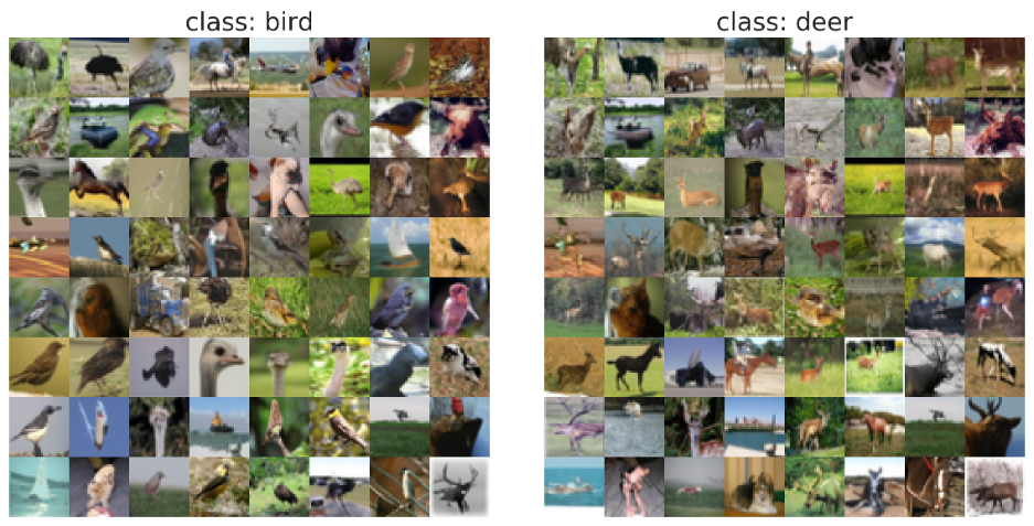
Below we show some examples on solving inverse problems for computer vision.

Connection to diffusion models and others

I started working on score-based generative modeling since 2019, when I was trying hard to make score matching scalable for training deep energy-based models on high-dimensional datasets. My first attempt at this led to the method sliced score matching. Despite the scalability of sliced score matching for training energy-based models, I found to my surprise that Langevin sampling from those models fails to produce reasonable samples even on the MNIST dataset. I started investigating this issue and discovered three crucial improvements that can lead to extremely good samples: (1) perturbing data with multiple scales of noise, and training score-based models for each noise scale; (2) using a U-Net architecture (we used RefineNet since it is a modern version of U-Nets) for the score-based model; (3) applying Langevin MCMC to each noise scale and chaining them together. With those methods, I was able to obtain the state-of-the-art Inception Score on CIFAR-10 in (even better than the best GANs!), and generate high-fidelity image samples of resolution up to $256\times 256$ in .

The idea of perturbing data with multiple scales of noise is by no means unique to score-based generative models though. It has been previously used in, for example, simulated annealing, annealed importance sampling, diffusion probabilistic models, infusion training, and variational walkback for generative stochastic networks. Out of all these works, diffusion probabilistic modeling is perhaps the closest to score-based generative modeling. Diffusion probabilistic models are hierachical latent variable models first proposed by Jascha and his colleagues in 2015, which generate samples by learning a variational decoder to reverse a discrete diffusion process that perturbs data to noise. Without awareness of this work, score-based generative modeling was proposed and motivated independently from a very different perspective. Despite both perturbing data with multiple scales of noise, the connection between score-based generative modeling and diffusion probabilistic modeling seemed superficial at that time, since the former is trained by score matching and sampled by Langevin dynamics, while the latter is trained by the evidence lower bound (ELBO) and sampled with a learned decoder.

In 2020, Jonathan Ho and colleagues significantly improved the empirical performance of diffusion probabilistic models and first unveiled a deeper connection to score-based generative modeling. They showed that the ELBO used for training diffusion probabilistic models is essentially equivalent to the weighted combination of score matching objectives used in score-based generative modeling. Moreover, by parameterizing the decoder as a sequence of score-based models with a U-Net architecture, they demonstrated for the first time that diffusion probabilistic models can also generate high quality image samples comparable or superior to GANs.

Inspired by their work, we further investigated the relationship between diffusion models and score-based generative models in an ICLR 2021 paper . We found that the sampling method of diffusion probabilistic models can be integrated with annealed Langevin dynamics of score-based models to create a unified and more powerful sampler (the Predictor-Corrector sampler). By generalizing the number of noise scales to infinity, we further proved that score-based generative models and diffusion probabilistic models can both be viewed as discretizations to stochastic differential equations determined by score functions. This work bridges both score-based generative modeling and diffusion probabilistic modeling into a unified framework.

Collectively, these latest developments seem to indicate that both score-based generative modeling with multiple noise perturbations and diffusion probabilistic models are different perspectives of the same model family, much like how wave mechanics and matrix mechanics are equivalent formulations of quantum mechanics in the history of physicsGoes without saying that the significance of score-based generative models/diffusion probabilistic models is in no way comparable to quantum mechanics.. The perspective of score matching and score-based models allows one to calculate log-likelihoods exactly, solve inverse problems naturally, and is directly connected to energy-based models, Schrödinger bridges and optimal transport. The perspective of diffusion models is naturally connected to VAEs, lossy compression, and can be directly incorporated with variational probabilistic inference. This blog post focuses on the first perspective, but I highly recommend interested readers to learn about the alternative perspective of diffusion models as well (see a great blog by Lilian Weng).

Many recent works on score-based generative models or diffusion probabilistic models have been deeply influenced by knowledge from both sides of research (see a website curated by researchers at the University of Oxford). Despite this deep connection between score-based generative models and diffusion models, it is hard to come up with an umbrella term for the model family that they both belong to. Some colleagues in DeepMind propose to call them “Generative Diffusion Processes”. It remains to be seen if this will be adopted by the community in the future.

Concluding remarks

This blog post gives a detailed introduction to score-based generative models. We demonstrate that this new paradigm of generative modeling is able to produce high quality samples, compute exact log-likelihoods, and perform controllable generation for inverse problem solving. It is a compilation of several papers we published in the past few years. Please visit them if you are interested in more details:

• Yang Song*, Sahaj Garg*, Jiaxin Shi, and Stefano Ermon. Sliced Score Matching: A Scalable Approach to Density and Score Estimation. UAI 2019 (Oral)

• Yang Song, and Stefano Ermon. Generative Modeling by Estimating Gradients of the Data Distribution. NeurIPS 2019 (Oral)

• Yang Song, and Stefano Ermon. Improved Techniques for Training Score-Based Generative Models. NeurIPS 2020

• Yang Song, Jascha Sohl-Dickstein, Diederik P. Kingma, Abhishek Kumar, Stefano Ermon, and Ben Poole. Score-Based Generative Modeling through Stochastic Differential Equations. ICLR 2021 (Outstanding Paper Award)

• Yang Song*, Conor Durkan*, Iain Murray, and Stefano Ermon. Maximum Likelihood Training of Score-Based Diffusion Models. NeurIPS 2021 (Spotlight)

• Yang Song*, Liyue Shen*, Lei Xing, and Stefano Ermon. Solving Inverse Problems in Medical Imaging with Score-Based Generative Models. ICLR 2022

For a list of works that have been influenced by score-based generative modeling, researchers at the University of Oxford have built a very useful (but necessarily incomplete) website: https://scorebasedgenerativemodeling.github.io/.

There are two major challenges of score-based generative models. First, the sampling speed is slow since it involves a large number of Langevin-type iterations. Second, it is inconvenient to work with discrete data distributions since scores are only defined on continuous distributions.

The first challenge can be partially solved by using numerical ODE solvers for the probability flow ODE with lower precision (a similar method, denoising diffusion implicit modeling, has been proposed in ). It is also possible to learn a direct mapping from the latent space of probability flow ODEs to the image space, as shown in . However, all such methods to date result in worse sample quality.

The second challenge can be addressed by learning an autoencoder on discrete data and performing score-based generative modeling on its continuous latent space . Jascha’s original work on diffusion models also provides a discrete diffusion process for discrete data distributions, but its potential for large scale applications remains yet to be proven.

It is my conviction that these challenges will soon be solved with the joint efforts of the research community, and score-based generative models/ diffusion-based models will become one of the most useful tools for data generation, density estimation, inverse problem solving, and many other downstream tasks in machine learning.