Accelerating Natural Gradient with Higher-Order Invariance
An overview for our ICML 2018 paper, Accelerating Natural Gradient with Higher-Order Invariance. Natural gradient update loses its invariance due to the finite step size. In this paper, we study the invariance of natural gradient from the perspective of Riemannian geometry, and propose several new update rules to improve its invariance. Empirical results show that better invariance can result in faster convergence in several supervised learning, unsupervised learning and reinforcement learning applications.
Probabilistic models are important for inference and prediction in many areas of machine learning. In this post, we focus our discussion on parametric probabilistic models, e.g., models that can be determined by specifying its parameters. Such a model may have several different parameterizations. For illustrative purposes, let’s consider a simple linear regression model that captures the joint distribution of input \(x\) and label \(y\):
\[p_\theta(x, y) = p(x) \mathcal{N}(y \mid \theta x + b, \sigma^2), \theta \in \mathbb{R},\]where \(\theta\) is the parameter, and \(b, \sigma\) are two fixed constants. By substituing \(\theta\) with \(2\mu\), a different parameterization can be created
\[p_\mu(x, y) = p(x) \mathcal{N}(y \mid 2\mu x + b, \sigma^2), \mu \in \mathbb{R}.\]Note that even if \(p_\theta(x,y)\) and \(p_\mu(x, y)\) have different analytical forms, they actually represent the same model family. In particular, \(p_{\theta=a}(x,y)\equiv p_{\mu=a/2}(x,y)\) for any \(a \in \mathbb{R}\).
Given a loss function \(L(p(x, y))\), the goal of an optimization algorithm is to find the model \(p^\ast(x, y)\) such that \(L(p^\ast(x, y))\) is as small as possible, in the form of finding the optimal parameter \(\theta^\ast\) or \(\mu^\ast\) under some parameterization. Although re-parameterization does not change the model family, the performance of optimization algorithms usually differs under different parameterizations. In the following section, we use the linear regression model as a running example to elaborate on why this can happen.
Why optimization can depend on parameterization
Returning to the example of linear regression, a typical loss function is the expected negative log-likelihood, which can be formally written as
\[\begin{aligned} L(p(x,y)) &= - \mathbb{E}_x [\log p(y\mid x)]\\ &= \mathbb{E}_x \left[\frac{1}{2\sigma^2} (\theta x + b - y)^2 + \log \sqrt{2\pi} \sigma \right] \quad \text{(for $p_\theta(x,y)$)}\\ &= \mathbb{E}_x \left[\frac{1}{2\sigma^2} (2\mu x + b - y)^2 + \log \sqrt{2\pi} \sigma \right] \quad \text{(for $p_\mu(x,y)$)} \end{aligned}\]Consider using gradient descent to minimize the loss function:
- For \(p_\theta(x,y)\), the update rule is \(\theta_{t+1} = \theta_t - \alpha \nabla_{\theta_t} L(p_{\theta_t}(x,y))\), where \(\alpha\) is the learning rate and
- For \(p_\mu(x,y)\), the update rule is \(\mu_{t+1} = \mu_{t} - \alpha \nabla_{\mu_t} L(p_{\mu_t}(x,y))\), where \(\alpha\) is the learning rate and gradient becomes
Let’s assume \(\theta_t = 2\mu_t = a\), i.e., at \(t\)-th optimization step, \(p_{\theta_t = a}(x,y)\) represents the same probabilistic model as \(p_{\mu_t = a/2}(x,y)\). However, because of this, the gradient has different scales:
\[\nabla_{\theta_t} L(p_{\theta_t}(x,y))\vert_{\theta_t = a} = \frac{1}{2} \nabla_{\mu_t} L(p_{\mu_t}(x,y))\vert_{\mu_t = a/2}\]and therefore
\[\begin{aligned} \theta_{t+1} &= \theta_{t} - \alpha \nabla_{\theta_t} L(p_{\theta_t}(x,y))\\ &= 2 \mu_t - \frac{\alpha}{2} \nabla_{\mu_t} L(p_{\mu_t}(x,y))\\ &\neq 2\mu_t - 2\alpha \nabla_{\mu_t} L(p_{\mu_t}(x,y))\\ &= 2\mu_{t+1}. \end{aligned}\]Hence the \((t+1)\)-th optimization step will result in different probabilistic models \(p_{\theta_{t+1}}(x,y) \not \equiv p_{\mu_{t+1}}(x,y)\). Specifically, one step of gradient descent will result in different models depending on which parameterization is used. This dependence on model parameterization can be undesirable, as it requires carefully choosing the parameterization to avoid hindering optimization.
For example, many tweaks are used to parameterize neural networks in such a way that they become more amenable to commonly used first-order optimization methods. We can view normalization methods of network activations, such as Batch Normalization
Luckily, this dependence on model parameterization is not universally true for every optimization method. For example, the Newton-Raphson method is invariant to affine transformations of model parameters. Therefore, for the linear regression case discussed above, the Newton-Raphson method will ensure that \(p_{\theta_{t+1}}(x,y) \equiv p_{\mu_{t+1}}(x,y)\) as long as \(p_{\theta_t}(x,y) \equiv p_{\mu_t}(x,y)\), because the new parameter \(\mu = \frac{1}{2}\theta\) is an affine transformation of \(\theta\).
Following this thread, we next discuss the Natural Gradient Method
Natural gradient method
From the example of applying gradient descent to linear regression, we can easily see that switching between model parameterizations can cause the gradients and parameters to change in different ways. So how can we ensure that when the parameterization changes, the gradient will also change in a clever way to compensate for its effect on these optimization algorithms?
In 1998, inspired by research on information geometry, Shun’ichi Amari proposed to use natural gradient
An Introduction to Riemannian Geometry
(click to expand or collapse)
The purpose of this text is to give readers the minimal background to understand the motivations behind natural gradient, invariance and our proposed improvements in the later part of this blog. For a more rigorous treatment on this topic, please refer to textbooks
Einstein summation convention
The convention states that
When any index variable appears twice in a term, once as a superscript and once as a subscript, it indicates summation of the term over all possible values of the index variable.
For example, \(a^\mu b_\mu := \sum_{\mu=1}^n a^\mu b_\mu\) when index variable \(\mu \in [n]\). Note that here the superscripts are not exponents but are indices of coordinates, coefficients or basis vectors. We will write the summation symbol \(\Sigma\) explicitly if we do not assume Einstein’s summation convention on some index, for instance, \(\sum_{\nu=1}^m a_\nu b_\nu c^\mu d_\mu := \sum_{\mu=1}^n \sum_{\nu=1}^m a_\nu b_\nu c^\mu d_\mu\).
Riemannian manifold
Riemannian geometry is used to study intrinsic properties of differentiable manifolds equipped with metrics. In machine learning, we often describe the space of some probabilistic models as a manifold. Informally, a manifold \(\mathcal{M}\) of dimension \(n\) is a smooth space whose local regions resemble \(\mathbb{R}^n\). Smoothness allows us to define a one-to-one local smooth mapping \(\phi: U \subset \mathcal{M} \rightarrow \mathbb{R}^n\) called chart or coordinate system, and for any \(p\in U\), \(\phi(p)\) represents the coordinates of \(p\). For instance, if \(p\) is a parameterized distribution, \(\phi(p)\) will refer to its parameters. Generally, manifolds may need a group of charts for complete description.
Tangent and cotangent spaces
Local resemblance to \(\mathbb{R}^n\) provides the foundation for defining a linear space attached to each point \(p \in \mathcal{M}\) called the tangent space \(\mathcal{T}_p\mathcal{M}\). Formally, \(\mathcal{T}_p\mathcal{M}=\{ \gamma'(0): \gamma \textrm{ is a smooth curve } \gamma:\mathbb{R} \rightarrow \mathcal{M}, \gamma(0)=p \}\) is the collection of all vectors obtained by differentiating smooth curves through \(p\), and consists of all tangent vectors to the manifold at point \(p\). Each tangent vector \(v \in \mathcal{T}_p\mathcal{M}\) can be identified with a directional differential operator acting on functions defined on \(\mathcal{M}\), with direction \(v\).
Let \(\phi(p) = (\theta^1,\theta^2,\cdots,\theta^n)\) be the coordinates of \(p\), it can be shown that the set of operators \(\{\frac{\partial}{\partial \theta^1},\cdots,\frac{\partial}{\partial \theta^n}\}\) forms a basis for \(\mathcal{T}_p\mathcal{M}\) and is called the coordinate basis. Note that \(\frac{\partial}{\partial \theta^\mu}\) is abbreviated to \(\partial_\mu\) and \(p\) is often identified with its coordinates \(\theta^\mu\) in the sequel.
Any vector space \(V\) has a corresponding dual vector space \(V^*\) consisting of all linear functionals on \(V\). The dual vector space of \(\mathcal{T}_p\mathcal{M}\) is called the cotangent space and is denoted \(\mathcal{T}_p^* \mathcal{M}\). Because \(\mathcal{T}_p\mathcal{M}\) is finite-dimensional, \(\mathcal{T}_p^* \mathcal{M}\) has the same dimension \(n\) as \(\mathcal{T}_p\mathcal{M}\). \(\mathcal{T}_p^* \mathcal{M}\) admits the dual coordinate basis \(\{d\theta^1,\cdots,d\theta^n\}\). These two sets of bases satisfy \(d\theta^\mu(\partial_\nu) = \delta^\mu_\nu\) where \(\delta^\mu_\nu\) is the Kronecker delta. To gain some intuition, if \(V\) is the space of all \(n\)-dimensional column vectors, \(V^*\) can be identified with the space of \(n\)-dimensional row vectors.
Vectors and covectors are geometric objects that exist independently of the coordinate system. Although their geometric properties do not depend on the basis used, their representation (in terms of coefficients) is of course basis-dependent. In particular, a change in the coordinate system (e.g., switching from Cartesian to polar coordinates) around \(p\) will alter the coordinate basis of \(\mathcal{T}_p\mathcal{M}\), resulting in transformations of coefficients of both vectors and covectors. Let the new chart be \(\phi'\) and let \(\phi(p) = (\theta^1,\cdots,\theta^n), \phi'(p) = (\xi^1,\cdots,\xi^n)\). The new coefficients of \(\mathbf{a} \in \mathcal{T}_p\mathcal{M}\) will be given by
\[a^{\mu'} \partial_{\mu'} = a^\mu \partial_\mu = a^\mu \frac{\partial \xi^{\mu'}}{\partial \theta^\mu} \partial_{\mu'} \Rightarrow a^{\mu'} = a^\mu \frac{\partial \xi^{\mu'}}{\partial \theta^\mu},\]while the new coefficients of \(\mathbf{a}^* \in \mathcal{T}_p^*\mathcal{M}\) will be determined by
\[a_{\mu'} d\xi^{\mu'} = a_\mu d\theta^\mu = a_\mu \frac{\partial \theta^\mu}{\partial \xi^{\mu'}} d\xi^{\mu'} \Rightarrow a_{\mu'} = a_\mu \frac{\partial \theta^\mu}{\partial \xi^{\mu'}}.\]Due to the difference in transformation rules, we call \(a^\mu\) to be contravariant while \(a_\mu\) covariant, as indicated by superscripts and subscripts respectively. For example, imagine a constant rescaling of the coordinates, such that all the new basis vectors are scaled by \(1/2\). To preserve the identity of a vector, its coefficients in this new basis will have to increase by a factor of \(2\) (changing contra-variantly with respect to the basis vectors). This means that the coefficients of a covector in the new basis will have to be scaled by \(1/2\) (changing co-variantly), so that it yields the same result when applied to a vector whose coefficients are twice as large in the new basis.
Riemannian manifolds are those equipped with a positive definite metric tensor \(g_p \in \mathcal{T}_p^* \mathcal{M} \otimes \mathcal{T}_p^* \mathcal{M}\). It is a symmetric bilinear positive definite scalar function of two vectors which defines the inner product structure of \(\mathcal{T}_p\mathcal{M}\), and makes it possible to define geometric notions such as angles and lengths of curves. Namely, the inner product of two vectors \(\mathbf{a} = a^\mu \partial_\mu \in \mathcal{T}_p\mathcal{M}\), \(\mathbf{b} = b^\nu \partial_\nu \in \mathcal{T}_p\mathcal{M}\) is defined as \(\langle \mathbf{a}, \mathbf{b} \rangle := g_p(\mathbf{a}, \mathbf{b}) = g_{\mu\nu} d \theta^\mu \otimes d\theta^\nu (a^\mu \partial_\mu, b^\nu\partial_\nu) = g_{\mu\nu} a^\mu b^\nu\). Here we drop the subscript \(p\) to avoid cluttering notations, although \(g_{\mu\nu}\) can depend on \(p\). For convenience, we denote the inverse of the metric tensor as \(g^{\alpha\beta}\) using superscripts, i.e., \(g^{\alpha\beta} g_{\beta\mu} = \delta^\alpha_\mu\).
The introduction of inner product induces a natural map from a tangent space to its dual. Let \(\mathbf{a} = a^\mu \partial_\mu \in \mathcal{T}_p\mathcal{M}\), its natural correspondence in \(\mathcal{T}_p^*\mathcal{M}\) is the covector \(\mathbf{a}^* := \langle \mathbf{a}, \cdot \rangle\). Let \(\mathbf{a}^* = a_\mu d\theta^\mu\), for any vector \(\mathbf{b} = b^\nu \partial_\nu \in \mathcal{T}_p\mathcal{M}\), we have \(\langle \mathbf{a}, \mathbf{b}\rangle = a^\mu b^\nu g_{\mu\nu} = \mathbf{a}^*(\mathbf{b}) = a_\mu d\theta^\mu(b^\nu \partial_\nu) = a_\mu b^\nu \delta^\mu_\nu = a_\mu b^\mu = a_\nu b^\nu\). Since the equation holds for arbitrary \(\mathbf{b}\), we have \(a_\nu = a^\mu g_{\mu\nu}\) and \(a^\mu = g^{\mu\nu}a_\nu\). Therefore the metric tensor relates the coefficients of a vector and its covector by lowering and raising indices.
Geodesics
Consider a curve \(\gamma(t): I \rightarrow \mathbb{R}^2\). Using Cartesian coordinates \(\gamma(t)=(x(t),y(t))\), it is easy to verify that \(\gamma\) is a straight line if it satisfies the following equation \(\frac{d^2 x}{d t} =\frac{d^2 y}{d t}=0\), i.e., \(x(t) = x_0 + v_x t, y(t) = y_0 + v_y t\). However, if we represent the curve using polar coordinates \(\gamma(t)=(r(t),\theta(t))\), i.e., \(x = r \cos \theta, y = r \sin \theta\), then \(\frac{d^2 r}{d t} =\frac{d^2 \theta}{d t}=0\) does not correspond to a straight line. The issue is that the coordinate basis depends on the position and will change as we move. For example, the radial directions \(\partial r\) at two points on a circle will be different.
We denote \(\nabla_{\mu} \partial_\nu\) as the vector describing how fast the basis \(\partial_\nu\) changes in the direction of \(\partial_\mu\). It is given by \(\nabla_{\mu} \partial_\nu = \Gamma_{\mu\nu}^\alpha \partial_\alpha\) where \(\Gamma_{\mu\nu}^\alpha\) is the connection, which specifies additional manifold structure associated with curvature and parallelness. Here we use the Levi-Civita connection which is defined in terms of the metric as
\[\Gamma_{\mu\nu}^\alpha = \frac{1}{2} g^{\alpha \beta}(\partial_\mu g_{\beta\nu} + \partial_\nu g_{\beta\mu} - \partial_\beta g_{\mu\nu}).\]A connection also specifies a way to transport a vector along a curve so that it stays parallel (to itself) with respect to the connection. Given the change rate of bases specified by the connection, the change rate of any vector \(\mathbf{a}\) along direction \(\mathbf{b}\) can be computed by
\[\nabla_{\mathbf{b}} \mathbf{a} = b^\mu \nabla_\mu (a^\nu \partial_\nu) = b^\mu (\partial_\mu a^\nu) \partial_\nu + b^\mu a^\nu \Gamma_{\mu\nu}^\alpha \partial_\alpha.\]We define the parallel transport of a vector \(\mathbf{a}\) along a curve \(\theta(t)\) as the solution to \(\nabla_{\dot \theta} \mathbf{a}(t) = 0\), where \(\dot \theta = \frac{d\theta}{dt}\) represents the tangent vector of \(\theta(t)\). This notion can be used to define the analogue of “straight lines’’, or geodesics, in general manifolds. A curve \(\theta(t)\) is a geodesic if the tangent vector \(\dot \theta = \frac{d\theta}{dt}\) is propagated parallelly to itself along the curve. This gives the geodesic equation \(\nabla_{\dot{\theta}} \dot{\theta} = 0\), or equivalently
\[\ddot\theta^\alpha + \Gamma_{\mu\nu}^\alpha \dot\theta^\mu \dot \theta^\nu = 0\]Note that \(\Gamma_{\mu\nu}^{\alpha}=0\) for \(\mathbb{R}^n\) with Euclidean metric and we recover usual straight lines. Let \(v \in \mathcal{T}_p\mathcal{M}\), there exists a unique geodesic satisfying \(\gamma(0)=p, \dot{\gamma}(0) = v\). This enables us to define the exponential map, i.e., \(\operatorname{Exp}(p,v) := \gamma(1)\). By simple scaling we also have \(\operatorname{Exp}(p, h v) = \gamma(h)\). Consistent with our intuition, geodesics (w.r.t. Levi-Civia connection) also correspond to local shortest paths between two points.
Summary
As a summary, we provide a graphical illustration of relevant concepts in Riemannian geometry.
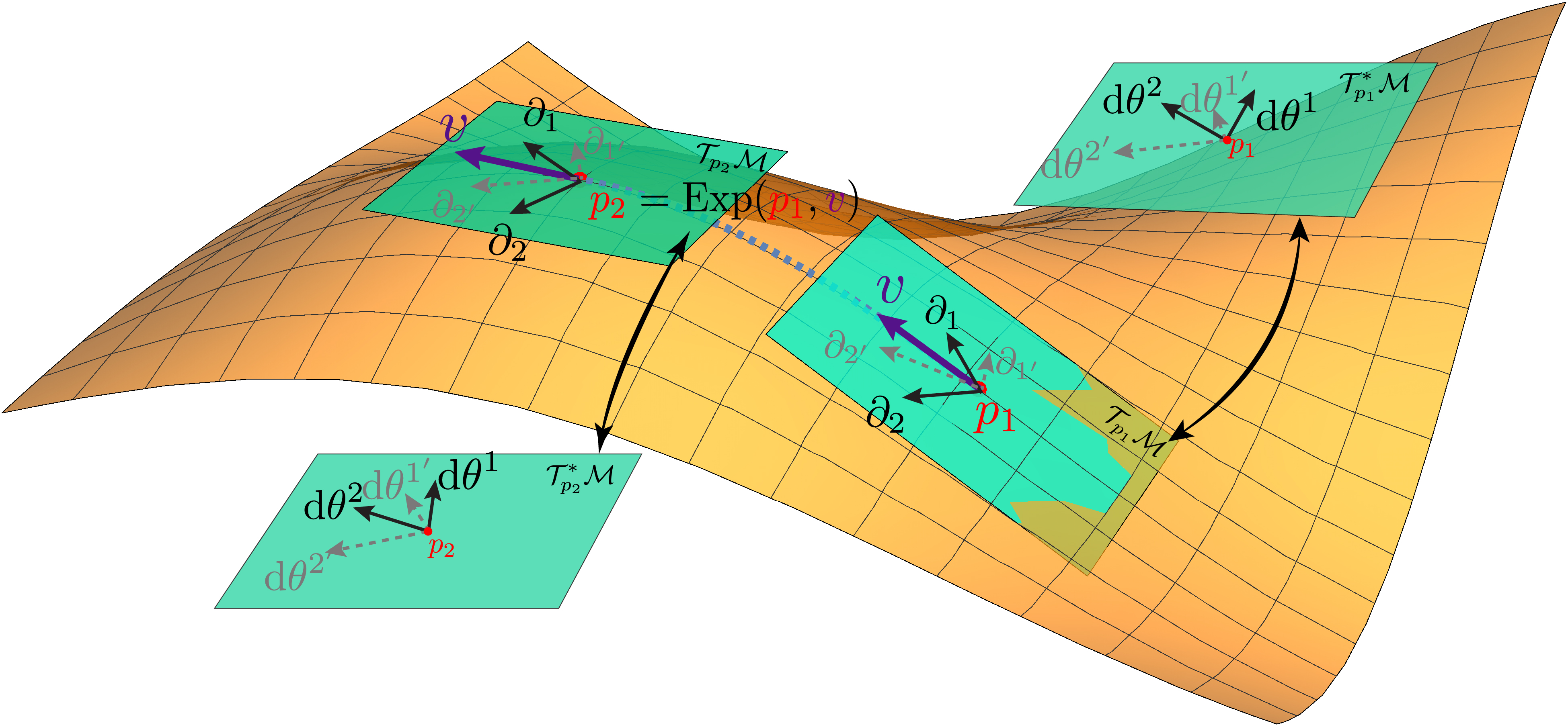
From the above formulation, we observe that every concept and relation is defined via coordinates or coefficients. However, we need to discern the important ontological difference between an object and its coordinate. The manifold itself, along with geodesics and vectors (covectors) in its tangent (cotangent) spaces is intrinsic and independent of coordinates provided by charts. Riemannian geometry studies intrinsic properties of manifolds via the lens of coordinates. As long as the coordinates are transformed accordingly, e.g., both transforms covariantly or contravariantly, the objects and their relations will not change. This is where invariance emerges.
Relation to natural gradient method
Let \(r_\theta(\mathbf{z}) = p_\theta(\mathbf{t}\mid\mathbf{x})q(\mathbf{x})\) be a probabilistic model parameterized by \(\theta \in \Theta\), and \(L(r_\theta) = - \mathbb{E}_{\mathbf{x}\sim q} [\log p_\theta(\mathbf{t}\mid\mathbf{x})]\) be the expected negative log-likelihood. Here \(\mathbf{x},\mathbf{t}\) are random variables, \(\mathbf{z} = (\mathbf{x},\mathbf{t})\) is their joint, \(q(\mathbf{x})\) is the marginal distribution of \(\mathbf{x}\) and is independent of \(\theta\). In a Riemannian geometry framework, the set of all possible models \(r_\theta\) constitutes a manifold \(\mathcal{M}\), and the parameter \(\theta\) provides a chart. Our goal is to find a model \(r_{\theta^*}\) that minimizes the (empirical) loss \(L(r_\theta)\), which is a function defined on the manifold.
The well known update rule of gradient descent \(\theta_{k+1}^\mu = \theta_k^\mu - h \lambda \partial_\mu L(r_{\theta_k})\) can be viewed as approximately solving the ordinary differential equation (ODE) \(\dot\theta^\mu = -\lambda \partial_\mu L(r_\theta)\) with forward Euler method. Here \(\lambda\) is a time scale constant, \(h\) is the step size, and their product \(h\lambda\) is the learning rate. However, the gradient descent ODE is not invariant to reparameterizations. For example, if we rescale \(\theta^\mu\) to \(2 \theta^\mu\), \(\partial_\mu L(r_\theta)\) will be downscaled to \(\frac{1}{2} \partial_\mu L(r_\theta)\). This is more evident from a differential geometric point of view. As can be verified by chain rules, \(\dot\theta^\mu\) transforms contravariantly and therefore is a vector in \(\mathcal{T}_p\mathcal{M}\), while \(\partial_\mu L(r_\theta)\) transforms covariantly, thus being a covector in \(\mathcal{T}^*_p\mathcal{M}\). Accordingly, the l.h.s. and r.h.s. of the ODE transform with different rules and do not type check. As a result, optimizing \(L(r_\theta)\) with gradient descent is using a parameterization-dependent method to solve a parameterization-independent problem, which is aesthetically unsatisfying.
Natural gradient alleviates this issue by approximately solving an invariant ODE. Recall that we can raise or lower an index given a metric tensor \(g_{\mu\nu}\), and hereby we choose the Fisher information metric given by
\[g_{\mu\nu} = \mathbb{E}_{\mathbf{x}\sim q} \mathbb{E}_{p_\theta(\mathbf{t}\mid\mathbf{x})}[\partial_\mu\log p_\theta(\mathbf{t}\mid\mathbf{x})\partial_\nu \log p_\theta(\mathbf{t}\mid\mathbf{x})].\]By raising the index of \(\partial_\mu L(r_\theta)\), the r.h.s. of the gradient descent ODE becomes a vector in \(\mathcal{T}_p\mathcal{M}\) and both sides transform contravariantly. The new invariant ODE is now \(\dot\theta^\mu = - \lambda g^{\mu\nu} \partial_\nu L(r_\theta)\), and the forward Euler approximation becomes \(\theta_{k+1}^\mu = \theta_k^\mu - h \lambda g^{\mu\nu}\partial_\nu L(r_{\theta_k})\), which is the traditional natural gradient update.
Intuitively, natural gradient is not the gradient with respect to model parameters; rather, it is the gradient on the manifold of probabilistic models. As opposed to the traditional gradient which considers how perturbations of the model parameters affect the loss function, natural gradient considers how the loss function changes when the probabilistic model moves a little bit on the manifold of our model family. Because the model family does not change with respect to parameterizations, the natural gradient will also remain the same. This means that the form of the natural gradient will transform appropriately between parameterizations, automatically ensuring that the natural gradient under two different parameterizations correspond to the same “gradient entity” on the manifold.
Mathematically, suppose the loss function is \(L(p_\theta(x,y))\), we can write the natural gradient as
\[\widetilde{\nabla}_\theta L(p_\theta(x,y)) := \mathbf{F}^{-1}_\theta \nabla_\theta L(p_\theta(x, y)),\]where \(\mathbf{F}_\theta\) is the Fisher information matrix for \(p_\theta(x, y)\), i.e.,
\[[\mathbf{F}_\theta]_{i,j} := \mathbb{E}_{p_\theta(x, y)} \left[\left( \frac{\partial}{\partial \theta_i} \log p_\theta(x,y)\right) \left( \frac{\partial}{\partial \theta_j} \log p_\theta(x,y) \right) \right],\]and we use a tilde mark (~) to differentiate the notation of natural gradient from that of ordinary gradient.
As a sanity check, let’s see how natural gradient eliminates the non-invariance of gradient descent for our linear regression example. For different parameterizations of Gaussian conditional distributions, the derivatives of the log densities are respectively
\[\begin{aligned} \frac{\partial}{\partial \theta} \log p_\theta(x,y) &= \frac{(y-\theta x- b) x}{\sigma^2}\\ \frac{\partial}{\partial \mu} \log p_\mu(x,y) &= \frac{2(y - 2\mu x -b) x}{\sigma^2}\\ \end{aligned}\]Therefore, suppose \(\theta_t = 2\mu_t = a\), we have \(\frac{\partial}{\partial \mu} \log p_\mu(x,y) \vert_{\mu=\mu_t} = 2 \frac{\partial}{\partial \theta} \log p_\theta(x,y)\vert_{\theta=\theta_t}\) and therefore \(\mathbf{F}_{\mu=\mu_t} = 4\mathbf{F}_{\theta=\theta_t}\). From our previous analysis on gradient descent, we already know that \(\nabla_\mu L(p_\mu(x, y))\vert_{\mu=\mu_t} = 2 \nabla_\theta L(p_\theta(x, y))\vert_{\theta_t=a}\). As a result, the natural gradient scales as
\[\widetilde{\nabla}_\mu L(p_\mu(x,y))\vert_{\mu=\mu_t} = \frac{1}{2}\widetilde{\nabla}_\theta L(p_\theta(x,y))\vert_{\theta=\theta_t},\]which indicates invariance of the optimization step:
\[\begin{aligned} \theta_{t+1} &= \theta_{t} - \alpha \widetilde{\nabla}_{\theta_t} L(p_{\theta_t}(x,y))\\ &= 2 \mu_t - 2 \alpha \widetilde{\nabla}_{\mu_t} L(p_{\mu_t}(x,y))\\ &= 2\mu_{t+1}. \end{aligned}\]More generally, consider an ordinary differential equation (ODE) that describes how the parameter \(\theta\) should change as a function of \(t\), following the natural gradient smoothly:
\[\frac{d \theta}{d t} = - \lambda \widetilde{\nabla}_\theta L(p_\theta(x,y))\]Here \(\lambda\) is just a prespecified scaling constant. If we change the parameterization from \(\theta\) to \(\mu\), we get a similar ODE:
\[\frac{d \mu}{d t} = - \lambda \widetilde{\nabla}_\mu L(p_\mu(x,y)).\]The following observation on invariance can be derived with knowledge of information theory and Riemannian geometry:
Suppose \(\mu\) is a smoothly differentiable transformation of \(\theta\). If \(p_{\theta(t=0)}(x,y) \equiv p_{\mu(t=0)}(x,y)\), and \(\theta(t)\), \(\mu(t)\) are solutions of corresponding natural gradient ODEs, then we have \(p_{\theta(t=a)}(x,y) \equiv p_{\mu(t=a)}(x,y)\) for any \(a \geq 0\).
However, it is usually intractable to solve such a complicated ODE for practical optimization tasks, and various approximation schemes must be used. From the perspective of numerical methods for ODEs, the naive natural gradient descent method
\[\theta_{t+1} = \theta_{t} - h \lambda \widetilde{\nabla}_{\theta_t} L(p_{\theta_t}(x,y))\]can be viewed as approximately solving the ODE
\[\frac{d \theta}{d t} = - \lambda \widetilde{\nabla}_\theta L(p_\theta(x,y))\]using the forward Euler method with a step size of \(h\). Such an approximation with discrete step size will potentially cause loss of invariance.
The following picture illustrates this point more clearly.
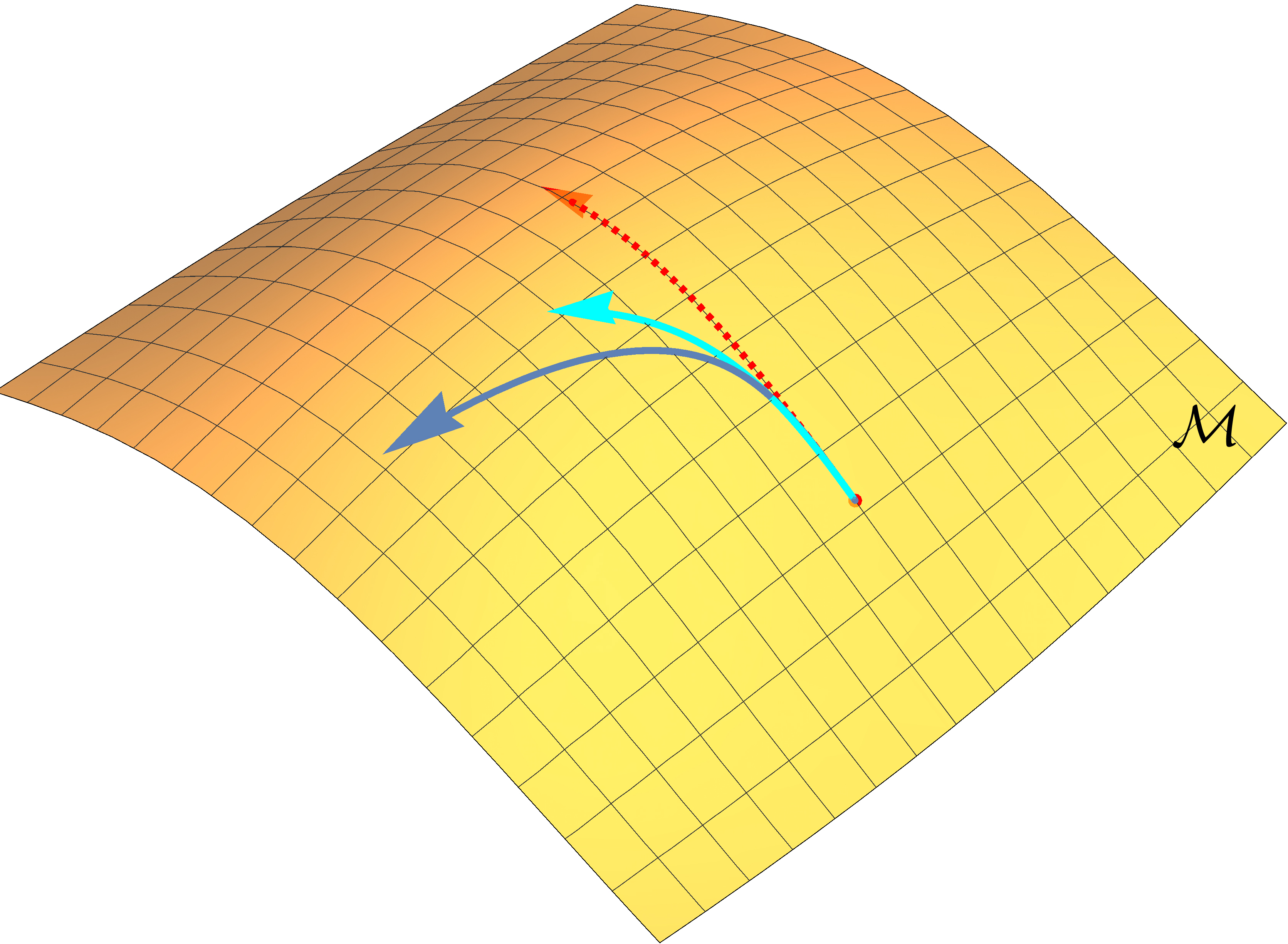
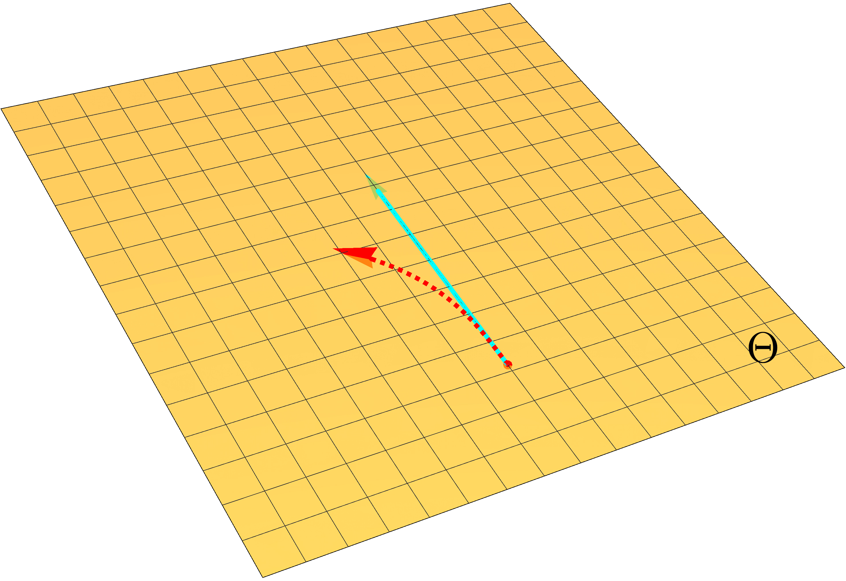
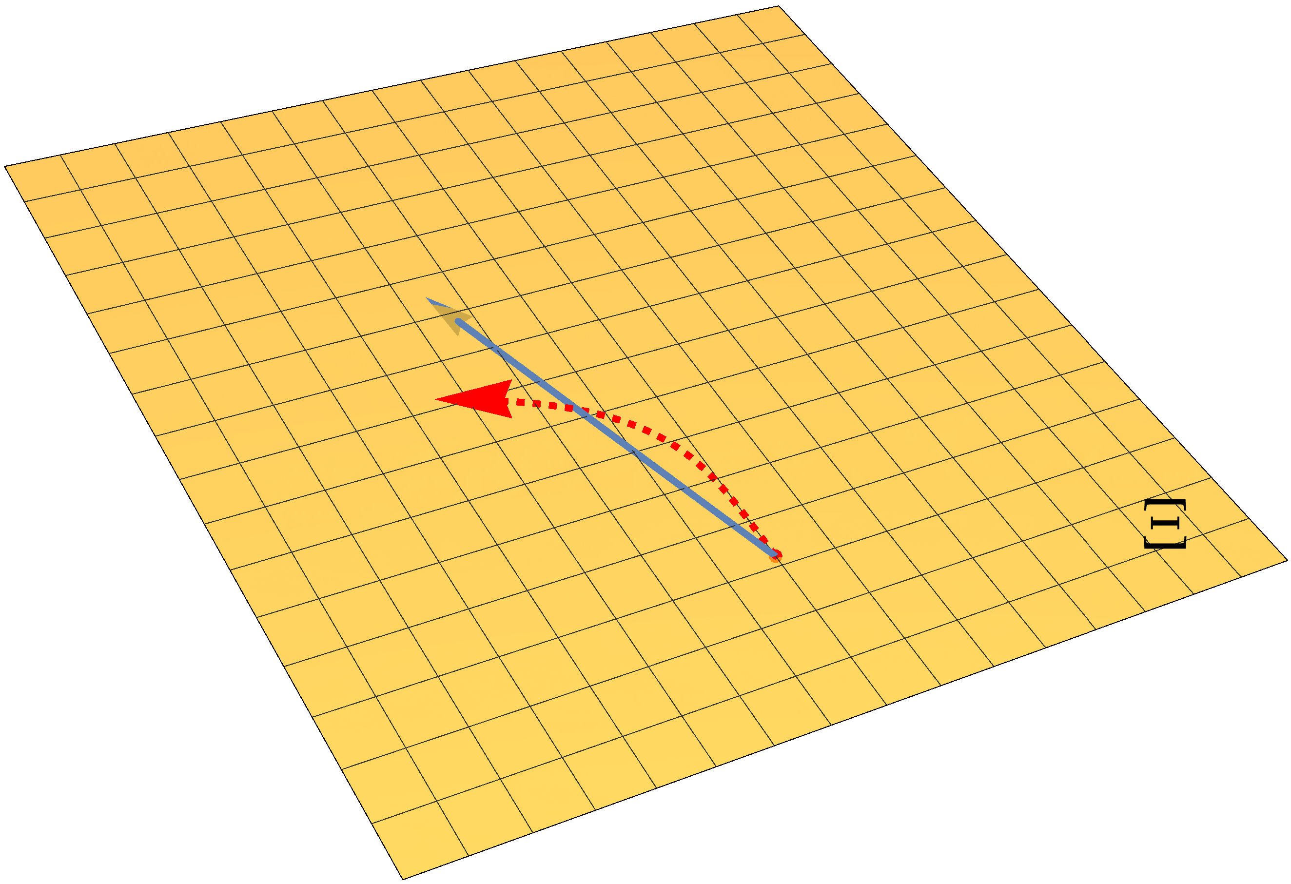
An illustration of optimization trajectories on the manifold (left), parameter space \(\Theta\) (middle) and another parameter space \(\Xi\) (right). The red dotted arrow represents a truly invariant trajectory, while the light and dark blue solid arrows represent trajectories of vanilla natural gradient updates under different parameterizations.
Suppose we are doing optimization on a manifold of probabilistic models \(\mathcal{M}\), and consider two different parameterizations with parameter spaces denoted as \(\Theta\) and \(\Xi\) respectively. The red arrow shows the invariant optimization trajectory obtained by accurately solving the natural gradient ODE. The light and dark blue arrows depict the optimization trajectory of the vanilla natural gradient descent under two different parameterizations.For the red arrows, we show the trajectory on manifold \(\mathcal{M}\), as well as trajectories in parameter space \(\Theta\) and \(\Xi\). For the blue arrows, we only show trajectories on \(\mathcal{M}\) and the parameter space.
Because vanilla natural gradient descent is a linear update, the blue trajectories in parameter space \(\Theta\) and \(\Xi\) are straight lines. However, in order to obtain the invariant trajectory (red arrow), the update has to be curved in parameter space. The update of the vanilla natural gradient descent is straight in the parameter space, and therefore its trajectory will not be truly invariant on \(\mathcal{M}\). For more invariant solutions, we need more complicated update rules that can perform curved updates in parameter space as well.
Because the natural gradient ODE solution is invariant, a straightforward approach to improving the invariance of the optimization is to exploit more accurate solvers. In numerical analysis, the accuracy of a solver is measured by computing its convergence order to the exact solution when step size \(h \rightarrow 0\). We say that a numerical ODE solver is \(d\)-th order accurate if the error between exact and approximate solutions decreases as \(O(h^d)\). The forward Euler solver used in the traditional natural gradient update is a simple first-order solver.
In a similar way, we can also measure the “invariance order” of a numerical ODE solver. We say that a solver is \(d\)-th order invariant if the error between the approximate solution and some exactly invariant trajectory decreases as \(O(h^d)\). Because the exact solution of the natural gradient ODE is invariant, any \(d\)-th order accurate solver is also \(d\)-th order invariant. We therefore have two ways to improve the invariance of natural gradient update — (1) using higher-order accurate solvers for the natural gradient ODE, or (2) using more invariant (but not necessarily more accurate) solvers.
Numerical ODE solvers that achieve better invariance
We discuss two approaches to improve the invariance of the natural gradient update:
1. More accurate solvers
Natural gradient ODE has an invariant solution; we just need to improve the accuracy of our numerical ODE solver such that the optimization trajectory is closer to the invariant one. In the paper, we discussed using a second-order solver called the Midpoint Method as a replacement for the first-order forward Euler method.
The Midpoint method can be decomposed into three steps to approximately solve the natural gradient ODE:
- Use gradient descent with half the step size to compute the midpoint: \(\theta_{t+1/2} = \theta_{t} - \frac{1}{2} h \lambda \widetilde{\nabla}_{\theta_t} L(p_{\theta_t}(x,y))\)
- Compute the gradient at the midpoint: \(\widetilde{\nabla}_{\theta_{t + 1/2}} L(p_{\theta_{t+1/2}}(x, y))\)
- Do the final update with the midpoint gradient: \(\theta_{t + 1} = \theta_{t} - h \lambda \widetilde{\nabla}_{\theta_{t+1/2}} L(p_{\theta_{t+1/2}}(x,y))\)
2. More invariant solvers
Some solvers can be more invariant by making their update rules more agonistic to reparameterizations, even though they are not necessarily more accurate than the forward Euler method. In the paper, we investigated a first-order solver called the Riemannian Euler Method
When applied to solving the natural gradient ODE, the Riemannian Euler method uses the following update rule:
\[\theta_{t+1} = \operatorname{Exp}(\theta_t, -h \lambda \widetilde{\nabla}_{\theta_t} L(p_{\theta_t}(x, y))),\]where \(\operatorname{Exp}(\cdot, \cdot)\) is the Exponential Map, a concept related to geodesics in Riemannian geometry. Unfortunately, evaluating \(\operatorname{Exp}(\cdot, \cdot)\) requires calculating geodesics on the manifold of probabilistic models, which is usually intractable.
The good news is that this exponential map can be easier to approximate than the invariant solution of the natural gradient ODE. Leveraging the geodesic equation—an ODE governing geodesic lines on a manifold—we can obtain a second-order approximation to the exponential map. Equipped with this approximation, the update rule now becomes
\[\begin{aligned} \gamma_t &= -\lambda \widetilde{\nabla}_{\theta_t} L(p_{\theta_t}(x,y))\\ \theta_{t+1} &= \underbrace{\theta_{t} + h \gamma_t}_{\text{naive natural gradient update}} \underbrace{- \frac{1}{2}h^2 \Gamma_{\theta_t}(\gamma_t,\gamma_t)}_{\text{geodesic correction}}. \end{aligned}\]Here \(\Gamma_{\theta_t}(\cdot, \cdot)\) represents the result of applying the Levi-Civita connection1 to input vectors. We name this update rule natural gradient update with geodesic correction.
An interesting observation is that if we use the naive natural gradient update rule, it amounts to using the Riemannian Euler method with first-order approximation to \(\operatorname{Exp}(\cdot, \cdot)\). This observation confirms that geodesic correction can provide more invariance (asymptotically).
The new numerical ODE solvers we explored so far are all computationally more expensive than the naive natural gradient update. For the midpoint integrator, we must calculate the midpoint first. For geodesic correction, we need to compute the Levi-Civita connection term. Both methods require about twice the computational cost compared to the naive natural gradient update. Luckily, we discovered that there exists a faster method for doing geodesic correction which still ensures a second-order approximation to the exponential map, presevering invariance. This faster geodesic correction is roughly as computationally expensive as the naive natural gradient update. Please refer to our paper for more details.
Overview of experimental results
Finally, we apply our techniques to improve the invariance of the natural gradient update and observe how they affect optimization performance. We first examine a toy problem to demonstrate that our methods achieve better invariance, then show that they lead to improved optimization for several tasks in various areas of machine learning, including supervised/unsupervised learning and reinforcement learning.
Testing invariance on a toy problem
We experiment with different natural gradient updates to fit a univariate Gamma distribution under different parameterizations. The canonical parameterization of a Gamma distribution is
\[p(x \mid \alpha, \beta) = \frac{\beta^\alpha}{\Gamma(\alpha)} x^{\alpha - 1} e^{-\beta x},\]where \(\Gamma(\cdot)\) denotes the Gamma function.
Aside from this canonical parameterization, we test three other parameterizations:
- Replacing \(\alpha\), \(\beta\) with \(\alpha'\), \(\frac{1}{\beta'}\).
- Replacing \(\alpha, \beta\) with \(\alpha', (\beta')^3\).
- Replacing \(\alpha, \beta\) with \((\alpha')^2, (\beta')^2\).
Next, we test all the natural gradient updates to see how well they can fit the parameters of a univariate Gamma distribution under different parameterizations. In the following figure, we show how the negative log-likelihood (our training loss) decreases with respect to training iterations. We use ng to denote the naive natural gradient update, mid for midpoint integrator, geo for geodesic correction, geof for the faster version of geodesic correction, ng(exact) for solving the natural gradient ODE exactly, and geo(exact) for using the exact Riemannian Euler method (without approximating the exponential map).
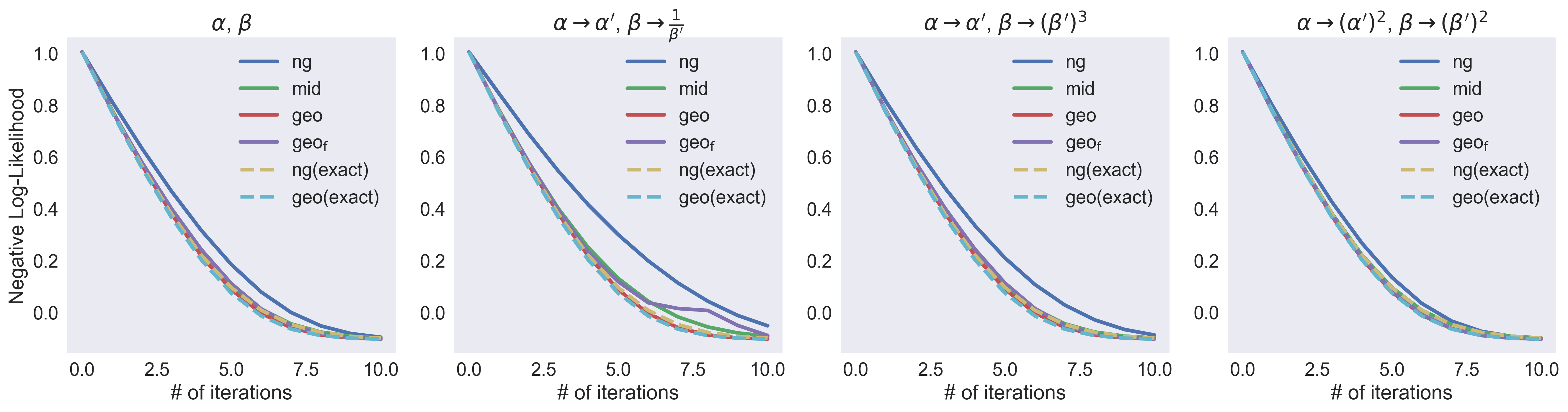
As the theory predicts, the curves of ng(exact) and geo(exact) are the same for all four different parameterizations. All of our proposed methods—mid, geo and geof—are closer to the exact invariant optimization curves. In stark contrast, the naive natural gradient update leads to different curves under different parameterizations, and yield slower convergence.
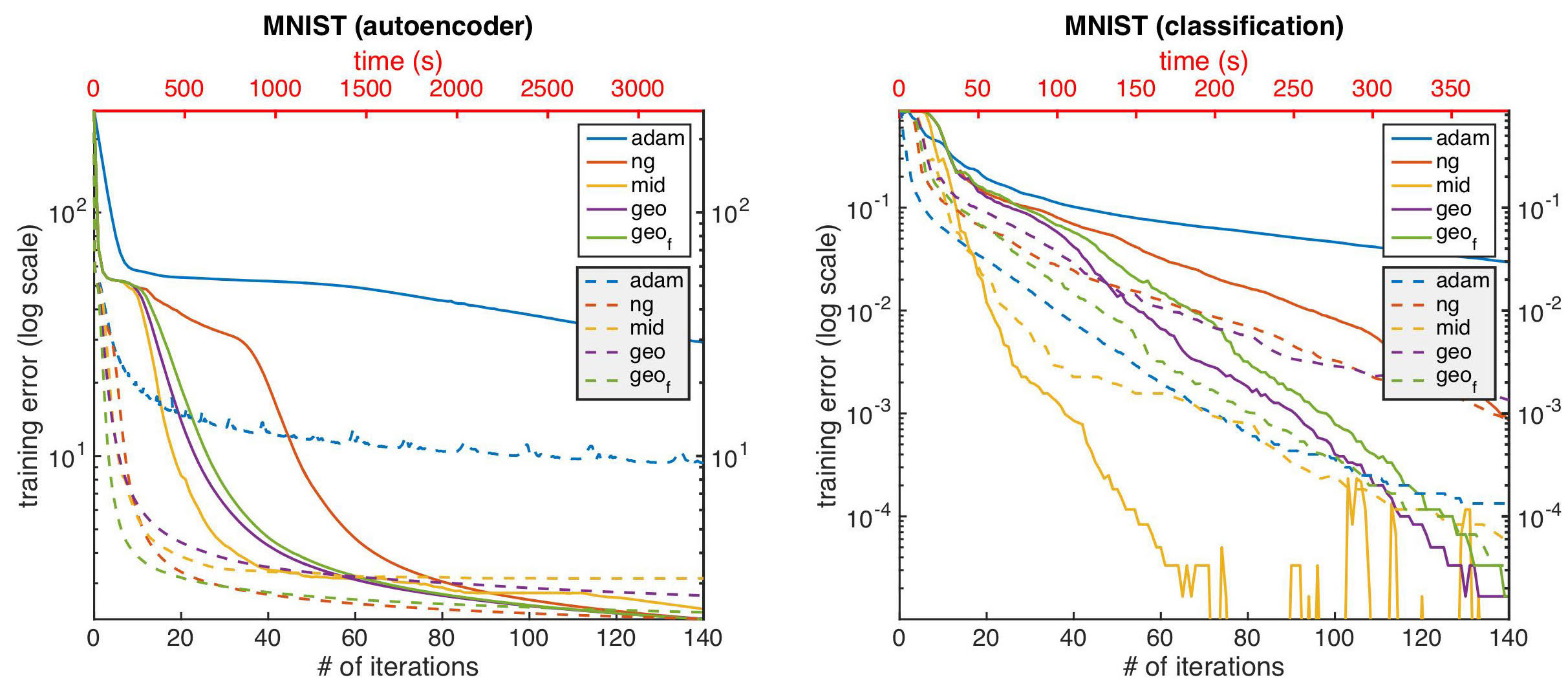
Fitting deep auto-encoders and deep classifiers
We then show the results of training deep autoencoders and classifiers on the MNIST dataset2. The following figure illustrates how the different optimization algorithms fare against each other. The bottom x-axis corresponds to the number of iterations during training, while the top x-axis corresponds to the wall-clock time. The y-axis shows the training error. Each optimization algorithm has two curves with the same color: one is solid while the other is dashed. We can observe that improved natural gradient updates converge faster in terms of number of iterations, and the faster geodesic correction also achieves lower loss in shorter wall-clock time, compared to the naive update.
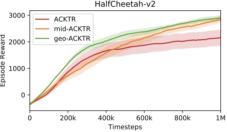
Model-free reinforcement learning for continuous control
Finally, we show that our techniques also improve the performance of natural gradient-based optimization algorithms in reinforcement learning. In the experiments, we apply our techniques to ACKTR
Conclusion
In this work, we analyze the invariance of optimization algorithms. Based on our analysis, we propose several methods to improve the invariance of natural gradient update. We empirically report that being more invariant leads to faster optimization for many machine learning tasks.
Footnotes
-
This is again a Riemannian geometry concept. The reader only needs to know that in practice \(\Gamma_{\theta_t}(\cdot, \cdot)\) can be computed almost as fast as \(\widetilde{\nabla}_{\theta_t} L(p_{\theta_t}(x,y))\). Please refer to the paper for more information. ↩
-
We also have results on 2 other datasets in the paper. ↩
-
We tested 5 other environments in the paper. ↩